Electric Dipole Moment, Electric Field on Axial and Equatorial Line of Electric Dipole and on axis of Uniformly Charged Ring with Numericals

This article provides a comprehensive explanation of the electric dipole and electric dipole moment, including their definition, properties, physical significance, direction, SI unit and dimensional formula. It also covers the electric field intensity due to an electric dipole at points on its axial and equatorial lines, the field due to a short dipole at any point, important derivations, formulas, special cases, and solved numerical problems. Along with detailed study material, the article includes downloadable PDF notes, Powerpoint pptx slideshow and a presentation video to support effective revision and examination preparation for CBSE Class 12 Physics, JEE Main, JEE Advanced and NEET.

Electric Dipole

An electric dipole consists of a pair of equal and opposite point charges separated by some small distance.

In Figure, we have shown two equal and opposite point charges +q, –q separated by a small distance 2a. It represents an electric dipole. 2a is called length of dipole. It can be taken as a vector whose direction is from negative charge to positive charge of dipole.

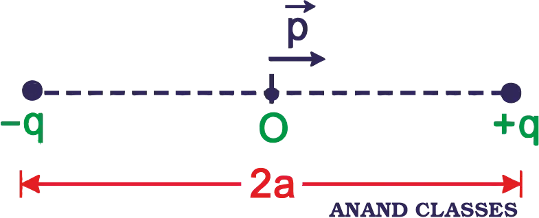
The middle point of locations of –q and +q is called the centre of the dipole. It is represented by O.

The total charge of the electric dipole = –q + q = 0.

This does not mean that the field of the electric dipole is zero.

Atoms or molecules of ammonia, water, alcohol, carbon dioxide, HCl etc. are some of the examples of electric dipoles, because in their cases, the centres of positive and negative charge distributions are separated by some small distance.

Figure shows a molecule of water (H₂O) with three nuclei represented by dots. The direction of electric dipole moment (p) points from the (negative) oxygen side to the (positive) hydrogen side of the molecule.

Frequently linked concepts include Electric Field Lines Properties, Electric Field due to Infinitely long thin wire, Charged Circular and Semicircular Ring

---

Dipole Moment

Dipole moment (p) is a measure of the strength of electric dipole. It is a vector quantity whose magnitude is equal to product of the magnitude of either charge and the distance between them.

Dipole moment = Either charge x a vector drawn from negative to positive charge

$\text{i.e., } \vec{p} = q(2\vec{a}) \quad \text{or} \quad \vert{}\vec{p}\vert{} = q(2a)$

Direction of Dipole Moment (p)

Dipole moment is a vector quantity and by convention, direction of dipole moment ($\vec{p}$) is from negative charge (-q) to positive charge (+q).

SI unit of dipole moment

The SI unit of dipole moment is coulomb-metre (Cm).

Dimensional formula of dipole moment

The dimensional formula of dipole moment is = [M⁰ L¹ A¹ T¹].

---

Ideal or Point Dipole

If charge q gets larger (q → ∞), and the distance 2a gets smaller and smaller (2a → 0), keeping the product p = q × 2a = finite value, we get what is called an ideal dipole or point dipole. Thus, an ideal dipole is the smallest dipole having almost no size.

Dipoles associated with individual atoms or molecules may be treated as ideal dipoles. An ideal dipole is specified only by its location and a dipole moment, as it has no finite size.

Strengthen your fundamentals with Electric Field due to Point Charge, Group of Charges, Continuous Charge Distribution Numerical Problems

---

Physical Significance of Electric Dipoles

The study of electric dipoles is important for electrical phenomena in matter. Matter, as we know, consists of atoms or molecules which are electrically neutral. In a molecule, there are positively charged nuclei and negatively charged electrons. If the centre of mass of positive charges coincides with the centre of mass of negative charges, the molecule behaves as a non-polar molecule.

On the contrary, if the centre of mass of positive charges does not coincide with the centre of mass of negative charges, the molecule behaves as a polar molecule and it possesses some intrinsic or permanent dipole moment. In the absence of an external electric field, the dipole moments of different molecules in a piece of matter are randomly oriented, so that net dipole moment of the piece is zero.

When an external electric field is applied, the polar molecules tend to align themselves along the field and some net dipole moment develops. The piece of matter is said to have been polarised.

When non-polar molecules are subjected to the action of an external electric field, the centres of mass of positive and negative charges in the molecule get displaced in opposite directions. Thus, the external field induces some dipole moment in the molecule in the direction of the field. The induced dipole moments of different molecules in the sample add up vectorially to produce some net total dipole moment.

---

Numerical Problems Based on Electric Dipole Moment for CBSE Class 12 Physics and JEE, NEET examinations

Practice these numerical problems to understand the calculation of electric dipole moment and its application in different electrostatic situations. These problems are useful for CBSE Class 12 Physics preparation and JEE, NEET examinations.

Charges ±20 nC are separated by 5 mm. Calculate the magnitude and direction of dipole moment.

Solution. Here q₁ = q₂ = q = ±20 nC = ±20 × 10^-9 C.

2a = 5 mm = 5 × 10^-3 m. The magnitude of dipole moment is as follows :

p = q (2a) = 20 × 10^-9 × 5 × 10^-3 = 10^-10 Cm

The direction of dipole moment (p) is from negative charge to positive charge.

Two charges, one +5 μC and another -5 μC are placed 1 mm apart. Calculate the dipole moment.

Solution. Here q = 5 μC = 5 × 10^-6 C, 2a = 1 mm = 10^-3 m
Dipole moment,

p = q × 2a

p = 5 × 10^-6 × 10^-3 = 5 × 10^-9 Cm

The direction of dipole moment (p) is from negative charge to positive charge.

Explore detailed notes on Forces Between Multiple Charges: Principle of Superposition Solved Numerical Problems

---

Electrostatics Complete Revision Notes PDF Download : Electric Dipole Moment and Its Applications

Download the Electrostatics Complete Revision Notes PDF on Electric Dipole Moment and Its Applications for comprehensive revision of important concepts in Class 12 Physics. These notes cover the definition and properties of an electric dipole, electric dipole moment, its direction, SI unit and dimensional formula, ideal or point dipole, physical significance of electric dipoles, and the electric field produced by a dipole at axial, equatorial and general points. The PDF also includes important derivations, formulas, solved numerical problems and key points useful for CBSE Class 12 Physics, JEE Main, JEE Advanced and NEET preparation. It is designed as a quick and useful study resource for revising the Electrostatics chapter before examinations.

To download the PDF notes of Electric Dipole Moment and Its Applications, click the Download PDF button below :

---

Dipole Field

The dipole field is the electric field produced by an electric dipole. It is the space around the dipole in which the electric effect of the dipole can be experienced. The electric field of the pair of charges (-q and +q) at any point in space can be found from Coulomb’s law and the superposition principle.

To calculate dipole field intensity at any point, we imagine a unit positive charge held at that point. We calculate force on this charge due to each charge of the dipole and take vector sum of the two forces. This gives us dipole field intensity at that point.

We shall show that though the total charge of electric dipole is zero, the field of the electric dipole is not zero. This is because the charges q and –q are separated by some distance. The electric fields due to these charges, when added, do not cancel out.

However, at distances much larger than the separation of two charges, i.e., r >> 2a, the fields due to q and –q largely cancel out. Therefore, at large distances from the dipole, the dipole field falls off more rapidly like E ∝ 1/r³ than like E ∝ 1/r² for a point charge.

---

Electric Field Intensity at any Point on Axial Line of Electric Dipole

Consider an electric dipole consisting of two point charges –q and +q separated by a small distance AB = 2a with centre at O and dipole moment, p = q(2a). We have to calculate electric intensity $\vec{E}$ at a point P on the axial line of the dipole, and at a distance OP = r from the centre O of the dipole as shown in Figure.

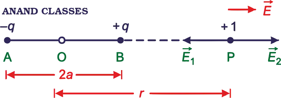
If $\vec{E}_1$ is the electric intensity at P due to charge –q, at A, then

$\vert{}\vec{E}_1\vert{} = \dfrac{1}{4\pi\epsilon_0} \dfrac{q}{AP^2}$

$\vert{}\vec{E}_1\vert{} = \dfrac{1}{4\pi\epsilon_0} \dfrac{q}{(r+a)^2}$

The direction of $\vec{E}_1$ electric intensity at P due to charge –q is along PA.

Suppose $\vec{E}_2$ is the electric intensity at P due to charge +q at B, then

$\vert{}\vec{E}_2\vert{} = \dfrac{1}{4\pi\epsilon_0} \dfrac{q}{BP^2}$

$\vert{}\vec{E}_2\vert{} = \dfrac{1}{4\pi\epsilon_0} \dfrac{q}{(r-a)^2}$

The direction of $\vec{E}_2$ is the electric intensity at P due to charge +q at B is along BP produced.

As $\vec{E}_1$ and $\vec{E}_2$ are collinear vectors acting in opposite directions and $\vert{}\vec{E}_2\vert{} > \vert{}\vec{E}_1\vert{}$, therefore, the resultant intensity $\vec{E}$ at P will be difference of two, acting along BP produced.

$\vert{}\vec{E}\vert{} = \vert{}\vec{E}_2\vert{} – \vert{}\vec{E}_1\vert{}$

$\vert{}\vec{E}\vert{} = \dfrac{1}{4\pi\epsilon_0} \dfrac{q}{(r-a)^2} – \dfrac{1}{4\pi\epsilon_0} \dfrac{q}{(r+a)^2}$

$\vert{}\vec{E}\vert{} = \dfrac{q}{4\pi\epsilon_0} \left[ \dfrac{1}{(r-a)^2} – \dfrac{1}{(r+a)^2} \right]$

$\vert{}\vec{E}\vert{} = \dfrac{q}{4\pi\epsilon_0} \left[ \dfrac{(r+a)^2 – (r-a)^2}{(r^2 – a^2)^2} \right]$

$\vert{}\vec{E}\vert{} = \dfrac{q}{4\pi\epsilon_0} \dfrac{4ar}{(r^2 – a^2)^2}$

$\vert{}\vec{E}\vert{} = \dfrac{q \times 2a \times 2r}{4\pi\epsilon_0 (r^2 – a^2)^2}$

But q × 2a = $\vert{}\vec{p}\vert{}$, the dipole moment. Therefore,

$\vert{}\vec{E}\vert{} = \dfrac{\vert{}\vec{p}\vert{}}{4\pi\epsilon_0} \dfrac{2r}{(r^2 – a^2)^2}$

If dipole is short, 2a << r,

$\vert{}\vec{E}\vert{} = \dfrac{\vert{}\vec{p}\vert{}}{4\pi\epsilon_0} \dfrac{2r}{r^4}$

$\vert{}\vec{E}\vert{} = \dfrac{2\vert{}\vec{p}\vert{}}{4\pi\epsilon_0 r^3}$

$\vert{}\vec{E}\vert{} = \dfrac{1}{4\pi\epsilon_0} \dfrac{2\vert{}\vec{p}\vert{}}{r^3}$

The direction of resultant electric field intensity $\vec{E}$ at point P due to electric dipole is along BP produced, i.e., along the direction of $\vec{p}$.

Clearly, $\vert{}\vec{E}\vert{} \propto \dfrac{1}{r^3}$

Noteworthy Point for Physics Class 12, JEE, NEET MCQ
Clearly, electric field at any axial point of the dipole acts along the dipole axis from negative to positive charge i.e., in the direction of dipole moment.

---

Numerical Problems Based on Electric Field Intensity at any Point on Axial Line of Electric Dipole for CBSE Class 12 Physics and JEE, NEET examinations

Practice these numerical problems to understand the electric field intensity produced by an electric dipole at points on its axial line. The problems are useful for CBSE Class 12 Physics, JEE and NEET examination preparation.

Two point charges, each of 5 μC but opposite in sign, are placed 4 cm apart. Calculate the electric field intensity at a point distant 4 cm from the midpoint on the axial line of the dipole.

Solution. Here q = 5 × 10^-6 C,

2a = 0.04 m, a = 0.02{ m, r = 0.04 m

$E_{\text{axial}} = \dfrac{1}{4\pi\varepsilon_0} \dfrac{2pr}{(r^2 – a^2)^2}$

$E_{\text{axial}} = \dfrac{1}{4\pi\varepsilon_0} \dfrac{2(q \times 2a)r}{(r^2 – a^2)^2}$

$E_{\text{axial}} = \dfrac{9 \times 10^9 \times 2 \times 5 \times 10^{-6} \times 0.04 \times 0.04}{[(0.04)^2 – (0.02)^2]^2}$

E_axial = 10⁸ NC^-1

The force experienced by a unit charge when placed at a distance of 0.10 m from the middle of an electric dipole on its axial line is 0.025 N and when it is placed at a distance of 0.2 m, the force is reduced to 0.002 N. Calculate the dipole length.

Solution. Electric Field Intensity at any Point on Axial Line of Electric Dipole

$E_{\text{axial}} = \dfrac{1}{4\pi\varepsilon_0} \cdot \dfrac{2pr}{(r^2 – a^2)^2}$

In first case: r = 0.10 m, E_axial = 0.025 N, therefore

$0.025 = \dfrac{9 \times 10^9 \times 2p \times 0.10}{[(0.10)^2 – a^2]^2}$

In second case: r = 0.2 m, E_axial = 0.002 N, therefore

$0.002 = \dfrac{9 \times 10^9 \times 2p \times 0.2}{[(0.2)^2 – a^2]^2}$

Dividing the above equations in above two cases, we get

$\dfrac{0.025}{0.002} = \dfrac{0.10}{0.2} \cdot \dfrac{[(0.2)^2 – a^2]^2}{[(0.1)^2 – a^2]^2}$

$5 = \dfrac{0.04 – a^2}{0.01 – a^2}$

therefore a = 0.05 m

Dipole length = 2a = 0.10 m

Build strong concepts by studying Coulomb’s Law of Electrostatics: Formula, Vector Form, Examples & Numericals

---

Electric Field Intensity at any Point on Equatorial Line of Electric Dipole

Consider an electric dipole consisting of two point charges –q and +q separated by a small distance AB = 2a with centre at O and dipole moment, p = q(2a). We have to calculate electric intensity $\vec{E}$ at a point P on the equatorial line of the dipole, and at a distance OP = r from the centre O of the dipole as shown in Figure.

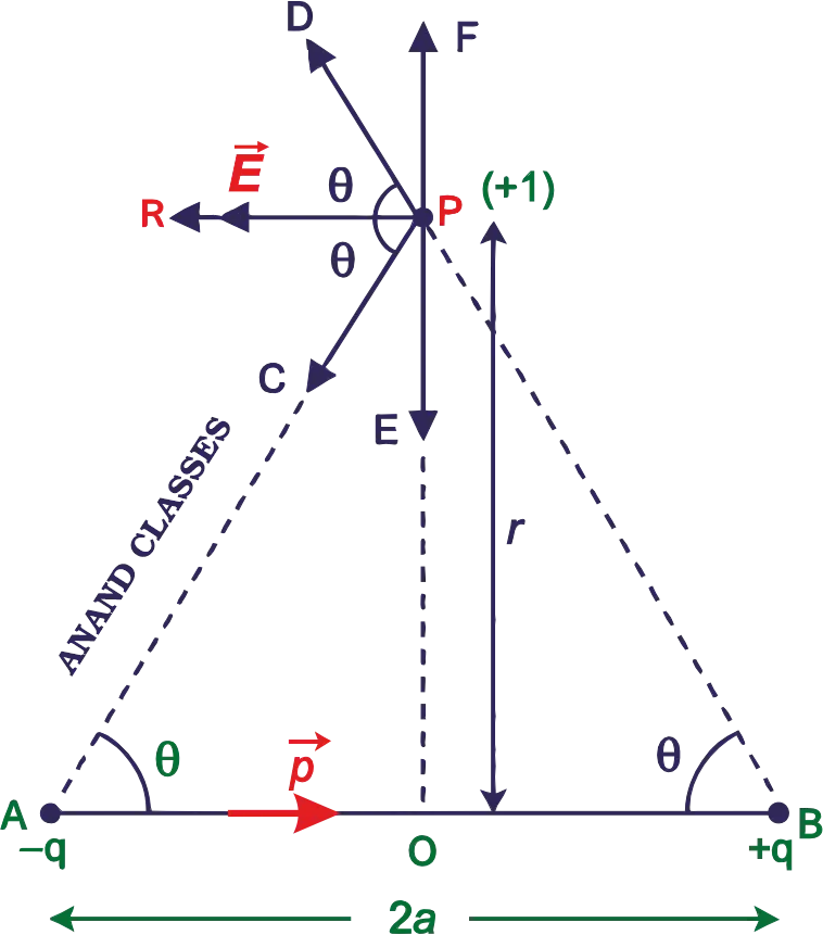
If $\vec{E}_1$ is electric intensity at P due to charge –q at A, then

$\vert{}\vec{E}_1\vert{} = \dfrac{1}{4\pi\epsilon_0} \dfrac{q}{AP^2}$

But, AP² = OP² + OA² = r² + a²

Therefore,

$\vert{}\vec{E}_1\vert{} = \dfrac{1}{4\pi\epsilon_0} \dfrac{q}{(r^2 + a^2)}$

$\vec{E}_1$ is represented by $\vec{PC}$.

Let ∠PBA = ∠PAB = θ.

$\vec{E}_1$ has two rectangular components:

• E₁ cos θ along PR ∥ BA
• E₁ sin θ along PE ⊥ BA

If $\vec{E}_2$ is electric intensity at P, due to charge +q at B, then

$\vert{}\vec{E}_2\vert{} = \dfrac{1}{4\pi\epsilon_0} \dfrac{q}{BP^2}$

$\vert{}\vec{E}_2\vert{} = \dfrac{1}{4\pi\epsilon_0} \dfrac{q}{(r^2 + a^2)}$

$\vec{E}_2$ is represented by $\vec{PD}$ (along BPD). $\vec{E}_2$ has two rectangular components :

• E₂ cos θ along PR ∥ BA
• E₂ sin θ along PF (opposite to PE)

As $\vert{}\vec{E}_1\vert{} = \vert{}\vec{E}_2\vert{}$, therefore E₁ sin θ along PE and E₂ sin θ along PF cancel out.

Therefore resultant intensity at P is given by

$\vert{}\vec{E}\vert{} = E_1 \cos\theta + E_2 \cos\theta$

$\vert{}\vec{E}\vert{} = 2 E_1 \cos\theta$

because $\vert{}\vec{E}_1\vert{} = \vert{}\vec{E}_2\vert{})$

$\vert{}\vec{E}\vert{} = \dfrac{2}{4\pi\epsilon_0} \dfrac{q}{(r^2 + a^2)} \cos\theta$

$\vert{}\vec{E}\vert{} = \dfrac{2}{4\pi\epsilon_0} \dfrac{q}{(r^2 + a^2)} \left( \dfrac{OA}{AP} \right)$

$\vert{}\vec{E}\vert{} = \dfrac{2}{4\pi\epsilon_0} \dfrac{q}{(r^2 + a^2)} \dfrac{a}{\sqrt{r^2 + a^2}}$

$\vert{}\vec{E}\vert{} = \dfrac{q \times 2a}{4\pi\epsilon_0 (r^2 + a^2)^{3/2}}$

But q × 2a = $\vert{}\vec{p}\vert{}$, the dipole moment

Therefore

$\vert{}\vec{E}\vert{} = \dfrac{\vert{}\vec{p}\vert{}}{4\pi\epsilon_0 (r^2 + a^2)^{3/2}}$

The direction of $\vec{E}$ is along PR ∥ BA (i.e., opposite to $\vec{p}$).

In vector form, we can rewrite resultant electric intensity equation as

$\vec{E} = \dfrac{-\vec{p}}{4\pi\epsilon_0 (r^2 + a^2)^{3/2}}$

Obviously, $\vec{E}$ is in a direction opposite to the direction of $\vec{p}$.

If the dipole is short, 2a << r, therefore

$\vert{}\vec{E}\vert{} = \dfrac{\vert{}\vec{p}\vert{}}{4\pi\epsilon_0 r^3}$

Clearly, $\vert{}\vec{E}\vert{} \propto \dfrac{1}{r^3}$

Noteworthy Point for Physics Class 12, JEE, NEET MCQ
Clearly, the direction of electric field at any point on the equatorial line of the dipole will be antiparallel to the direction of dipole moment p.

---

Numerical Problems Based on Electric Field Intensity at any Point on Equatorial Line of Electric Dipole for CBSE Class 12 Physics and JEE, NEET examinations

Practice these numerical problems to understand the electric field intensity produced by an electric dipole at points on its equatorial line. The problems are useful for CBSE Class 12 Physics, JEE and NEET examination preparation.

Calculate the electric field due to an electric dipole of length 10 cm having charges of 1 μC at an equatorial point 12 cm from the centre of the dipole.

Solution. Here q = 1 μC = 10^-6 C, r = 12 cm = 0.12 m,

2a = 10 cm, a = 5 cm = 0.05 m

$E_{\text{equatorial}} = \dfrac{1}{4\pi\varepsilon_0} \cdot \dfrac{2qa}{(r^2 + a^2)^{3/2}}$

$E_{\text{equatorial}} = \dfrac{9 \times 10^9 \times 2 \times 10^{-6} \times 0.05}{(0.12^2 + 0.05^2)^{3/2}}$

E_equatorial = 4.096 × 10⁵ NC^-1

---

Comparison of the magnitudes of Electric fields of a Short dipole at Axial and Equatorial Points

The magnitude of the electric field of a short dipole at an axial point at distance r from its centre is

$\vert{}\vec{E}\vert{} = \dfrac{1}{4\pi\epsilon_0} \dfrac{2\vert{}\vec{p}\vert{}}{r^3}$

Electric field at an equatorial point at the same distance r is

$\vert{}\vec{E}\vert{} = \dfrac{\vert{}\vec{p}\vert{}}{4\pi\epsilon_0 r^3}$

$\dfrac{E_{\text{axial}}}{E_{\text{equatorial}}} = 2$

$E_{\text{axial}}= 2 \times {E_{\text{equatorial}}}$

i.e., at a given distance from the centre of dipole, electric field intensity on axial line is twice the electric intensity on equatorial line. Further, both the magnitude and the direction of dipole field depend not only on the distance r, but also on the angle between the position vector $\vec{r}$ and dipole moment $\vec{p}$.

Note. Position on Axial Line of an electric dipole is also known as End on position. And position on equatorial line of an electric dipole is also known as Broadside on position.

---

Electric Field Intensity due to a Short Electric Dipole at an arbitrary point making an angle θ with the dipole axis

In Figure, AB represents a short electric dipole of moment $\vec{p}$ along AB. O is the centre of dipole. We have to calculate electric field intensity $\vec{E}$ at any point K, where OK = r, ∠BOK = θ.

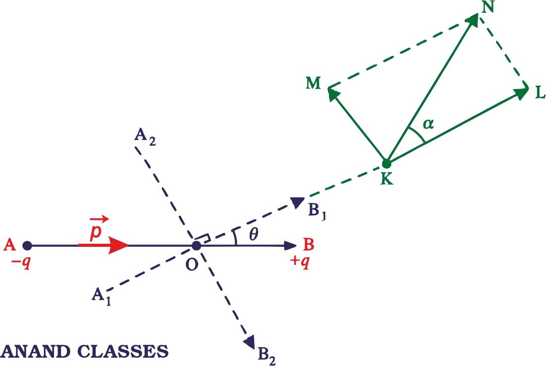
The dipole moment $\vec{p}$ can be resolved into two rectangular components :

• p cos θ along A₁ B₁
• p sin θ along A₂ B₂ ⊥ A₁ B₁

Field intensity at K on the axial line of A₁ B₁,

$\vert{}\vec{E}_1\vert{} = \dfrac{1}{4\pi\epsilon_0} \dfrac{2p \cos\theta}{r^3}$

Let it be represented by $\vec{KL}$ along OK.

Field intensity at K on equatorial line of A₂ B₂,

$\vert{}\vec{E}_2\vert{} = \dfrac{1}{4\pi\epsilon_0} \dfrac{p \sin\theta}{r^3}$

Let it be represented by $\vec{KM}$ ∥ B₂ A₂ and ⊥ $\vec{KL}$. Complete the rectangle KLNM. Join KN.

According to parallelogram law, KN represents resultant intensity ($\vec{E}$) at K due to the short dipole.

As $KN = \sqrt{KL^2 + KM^2}$. Therefore,

$\vert{}\vec{E}\vert{} = \sqrt{E_1^2 + E_2^2}$

$\vert{}\vec{E}\vert{} = \sqrt{\left( \dfrac{1}{4\pi\epsilon_0} \dfrac{2p \cos\theta}{r^3} \right)^2 + \left( \dfrac{1}{4\pi\epsilon_0} \dfrac{p \sin\theta}{r^3} \right)^2}$

$\vert{}\vec{E}\vert{} = \dfrac{p}{4\pi\epsilon_0 r^3} \sqrt{4\cos^2\theta + \sin^2\theta}$

$\vert{}\vec{E}\vert{} = \dfrac{p}{4\pi\epsilon_0 r^3} \sqrt{3\cos^2\theta + (\cos^2\theta + \sin^2\theta)}$

$\vert{}\vec{E}\vert{} = \dfrac{p}{4\pi\epsilon_0 r^3} \sqrt{3\cos^2\theta + 1}$

i.e., $\vert{}\vec{E}\vert{} = \dfrac{p \sqrt{3\cos^2\theta + 1}}{4\pi\epsilon_0 r^3}$

Let ∠LKN = α. In △KLN,

$\tan\alpha = \dfrac{LN}{KL}$

$\tan\alpha = \dfrac{KM}{KL}$

$\tan\alpha = \dfrac{\dfrac{p \sin\theta}{4\pi\epsilon_0 r^3}}{\dfrac{2p \cos\theta}{4\pi\epsilon_0 r^3}}$

$\tan\alpha = \dfrac{1}{2}\tan\theta$

Therefore, α can be calculated.

Special cases :

1. When the point K lies on axial line of dipole.

θ = 0°, cos θ = cos 0° = 1. Therefore,

$\vert{}\vec{E}\vert{} = \dfrac{p}{4\pi\epsilon_0 r^3} \sqrt{3\cos^2 0^\circ + 1}$

$\vert{}\vec{E}\vert{} = \dfrac{2p}{4\pi\epsilon_0 r^3}$

and tan α = 1/2 tan 0° = 0, therefore α = 0° i.e., resultant intensity is along the axial line.

2. When the point K lies on equatorial line of dipole.

θ = 90°, cos θ = cos 90° = 0. Therefore,

$E = \dfrac{p}{4\pi\epsilon_0 r^3} \sqrt{3\cos^2 90^\circ + 1}$

$E = \dfrac{p}{4\pi\epsilon_0 r^3}$

and tan α = 1/2 tan 90° = 1/0, therefore α = 90° i.e., direction of resultant field intensity is perpendicular to the equatorial line (and hence antiparallel to axial line of dipole).

To strengthen your concepts, learn about Electric Charge Quantization, Additivity, Charging by Induction, Solved Numericals

---

Numerical Problems Based on Electric Field Intensity at any Point due to Short Electric Dipole for CBSE Class 12 Physics and JEE, NEET examinations

Practice these numerical problems to understand the electric field intensity produced by an electric dipole at any point. The problems are useful for CBSE Class 12 Physics, JEE and NEET examination preparation.

Two charges ±10 μC are placed 5.0 mm apart. Determine the electric field at (a) a point P on the axis of dipole 15 cm away from its centre on the side of the positive charge, as shown in Figure and at (b) a point Q, 15 cm away from O on a line passing through O and normal to the axis of the dipole as shown in Figure. [NCERT Solved Example]

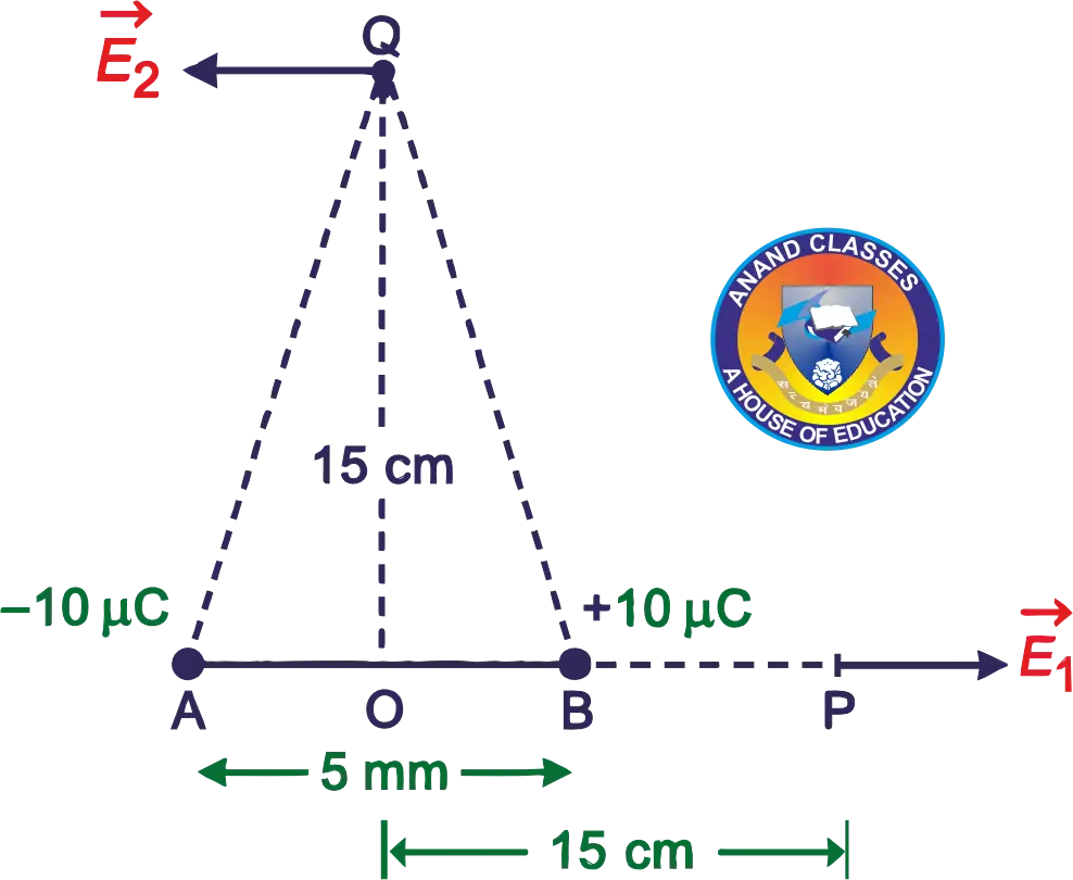
Solution. Here, q = ±10 μC = ±10^-5 C, 2a = 5.0 mm = 5 × 10^-3 m

r = OP = 15 cm = 15 × 10^-2 m. The electric dipole moment,

p = q × 2a

p = 10^-5 × 5 × 10^-3 = 5 × 10^-8 Cm

(a) As P lies on axial line of dipole, Therefore

$E_1 = \dfrac{2\vert{}\vec{p}\vert{}r}{4\pi\varepsilon_0 (r^2 – a^2)^2},$ along BP

As a << r, therefore,

$E_1 = \dfrac{2\vert{}\vec{p}\vert{}}{4\pi\varepsilon_0 \, r^3}$

$E_1 = \dfrac{2 \times 5 \times 10^{-8} \times 9 \times 10^9}{(15 \times 10^{-2})^3}$

E₁ = 2.67 × 10⁵ N/C, along BP

This field is directed along the direction of dipole moment vector, i.e., from –q to +q,

(b) As Q lies on equatorial line of dipole, therefore

$E_2 = \dfrac{\vert{}\vec{p}\vert{}}{4\pi\varepsilon_0 (r^2 + a^2)^{3/2}}$

$E_2 = \dfrac{\vert{}\vec{p}\vert{}}{4\pi\varepsilon_0 \, r^3}$, because a << r

$E_2 = \dfrac{1}{2} E_1 = \dfrac{1}{2} \times 2.67 \times 10^5$

E₂ = 1.33 × 10⁵ N/C, is along a line parallel to BA.

This field is directed opposite to the direction of the dipole moment vector, i.e., from +q to –q.

---

Electric Field Intensity at any Point on the axis of a Uniformly Charged Ring and Where Electric Field Intensity be Maximum

Consider a circular loop of wire of negligible thickness, radius a and centre O held perpendicular to the plane of the paper. Let the loop carry a total charge +q distributed uniformly over its circumference. We have to determine electric field intensity at any point P on the axis of the loop, where OP = r.

Consider a small element AB of the loop. Let length of element AB = dl and C be the centre of the element.

Charge on the element AB is

$dq = \dfrac{q}{2\pi a} dl$

Electric Field intensity at P due to the charge element AB is

$|d\vec{E}| = \dfrac{1}{4\pi\epsilon_0} \dfrac{dq}{CP^2}$

along PC‘ at angle θ with the axis OX.

$|d\vec{E}| = \dfrac{1}{4\pi\epsilon_0} \dfrac{dq}{(r^2 + a^2)}$

$d\vec{E}$ can be resolved into two rectangular components.

• dE cos θ along PX, the axis of the loop, and
• dE sin θ along PY, perpendicular to the axis.

For a pair of diametrically opposite elements of the loop, components of electric field intensity perpendicular to the axis will cancel, whereas the components along the axis of the loop will add. As the loop can be considered to be made up of a large number of pairs of diametrically opposite elements, therefore,

ΣdE sin θ = 0

Hence the resultant electric field intensity at P is

$|\vec{E}|$ = ΣdE cos θ

In △OPC,

$\cos\theta = \dfrac{OP}{CP}$

$\cos\theta = \dfrac{r}{(r^2 + a^2)^{1/2}}$.

Therefore, resultant electric field intensity at any point on the axis of a uniformly charged ring is as follows :

$|\vec{E}| = \sum \dfrac{1}{4\pi\epsilon_0} \dfrac{dq}{(r^2 + a^2)} \dfrac{r}{(r^2 + a^2)^{1/2}}$

$\vert{}\vec{E}\vert{} = \sum \dfrac{1}{4\pi\varepsilon_0} \left(\dfrac{q \, dl}{2\pi a}\right) \dfrac{r}{(r^2 + a^2)^{3/2}}$

$\vert{}\vec{E}\vert{} = \dfrac{q\,r}{4\pi\varepsilon_0 \, 2\pi a (r^2 + a^2)^{3/2}}\sum_{\text{whole loop}} dl$

$\vert{}\vec{E}\vert{} = \dfrac{q\,r (2\pi a)}{4\pi\varepsilon_0 \, 2\pi a (r^2 + a^2)^{3/2}}$

$\vert{}\vec{E}\vert{} = \dfrac{q\,r}{4\pi\varepsilon_0 (r^2 + a^2)^{3/2}}$

The direction of $\vec{E}$ is along PX, the axis of the loop.

Special Cases.

1. When P lies at the centre of the loop.

r = 0, therefore, $\vec{E}$ = 0

2. When r >> a (i.e. P lies far off from the loop), neglecting a² in comparison to r² in above equation, we get

$\vert{}\vec{E}\vert{} = \dfrac{q\,r}{4\pi\varepsilon_0 \, r^3}$

$\vert{}\vec{E}\vert{} = \dfrac{q}{4\pi\varepsilon_0 \, r^2},$ along PX

This is the expression for $\vec{E}$ at a distance r from a point charge q. Hence a circular loop of charge behaves as a point charge when the observation point (P) is at very large distance from the loop, compared to the radius of the loop.

3. Electric field intensity due to a uniformly charged ring will be maximum. When

$\dfrac{dE}{dr} = 0$

$\dfrac{d}{dr} \left[ \dfrac{q \times r}{4\pi\varepsilon_0 (r^2 + a^2)^{3/2}} \right] = 0$

$\dfrac{q}{4\pi\varepsilon_0} \left[ \dfrac{-3r^2}{(r^2 + a^2)^{5/2}} + (r^2 + a^2)^{-3/2} \right] = 0$

$\dfrac{3r^2}{(r^2 + a^2)^{5/2}} = (r^2 + a^2)^{-3/2}$

3r² = (r² + a²)

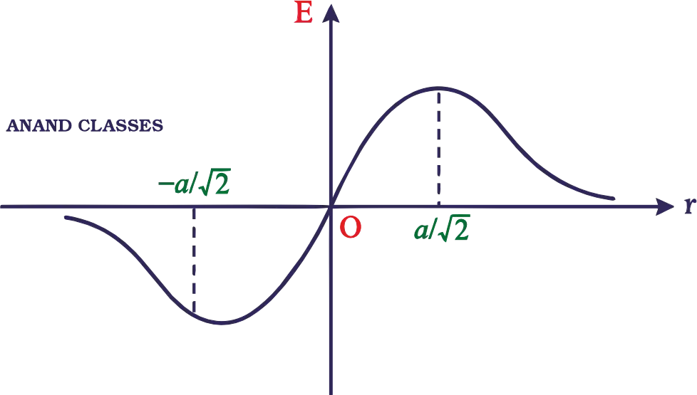
r = ± a/√2

Thus electric field intensity due to a uniformly charged ring will be maximum at a distance r = a/√2 from its centre on either side on the axis of the ring. The variation of electric field intensity due to a charged ring with the distance r from the centre of the ring is shown in Figure.

---

Conceptual Short Questions Answers Based on Electric Field Intensity on Axial and Equatorial Line of Electric Dipole

These conceptual short questions and answers help students understand the electric field intensity of an electric dipole on its axial and equatorial lines, including the direction, magnitude, and comparison of electric fields at different points.

A point charge placed at any point on the axis of an electric dipole at some large distance experiences a force F. What will be the force acting on the point charge when its distance from the dipole is doubled?

Answer. At any axial point of a dipole, electric field varies as

E ∝ 1/r³

F/q ∝ 1/r³

F ∝ 1/r³

When the distance of the point charge is doubled, the force reduces to F/8.

At what points, dipole field intensity is parallel to the line joining the charges ?

Answer. At any point on axial line or equatorial line of dipole.

---

Electrostatics Complete Revision Notes PPTX Slideshow Download: Electric Dipole Moment and Its Applications

This PowerPoint presentation (PPTX) provides a clear and systematic explanation of Electric Dipole Moment and Its Applications for Class 12 Physics students. The slideshow covers the concept of an electric dipole, electric dipole moment, its direction, SI unit and dimensional formula, ideal or point dipole, physical significance of electric dipoles, and electric field intensity at axial, equatorial and general points. It also includes important formulas, derivations, special cases, solved numerical problems and key concepts for effective revision. The presentation is particularly useful for CBSE Class 12 Physics, JEE Main, JEE Advanced and NEET examination preparation and helps students understand the relationship between electric dipole moment and the electric field produced by a dipole.

---

Electrostatics: Electric Dipole Moment and Its Applications Presentation Video

Watch this presentation video to understand the Electric Dipole Moment and its applications in a simple and systematic way. The presentation covers the concept of an electric dipole, dipole moment, its direction, SI unit and dimensional formula, along with the electric field produced by an electric dipole at points on its axial and equatorial lines. It also explains the electric field due to a short electric dipole, important special cases, key formulas and numerical applications. This presentation is useful for CBSE Class 12 Physics, JEE and NEET preparation and for strengthening your concepts of Electrostatics.

Topics covered: Electric Dipole, Electric Dipole Moment, Ideal Dipole, Dipole Field, Axial Position, Equatorial Position, Short Electric Dipole, Electric Field Intensity, Important Formulas and Solved Numerical Problems.