Electric Field due to Point Charge, Group of Charges, Continuous Charge Distribution Numerical Problems

Electric field is covered through its definition, intensity, direction and characteristics, followed by electric field due to point charges and groups of discrete charges. The discussion includes radial electric fields, the principle of superposition, force due to continuous charge distributions, and volume, surface and line charge distributions. Different methods of resolving electric field intensity into rectangular components are also included. The topic is further developed through solved numerical problems involving charged oil drops, charged pendulums, electrons and protons, parallel capacitor plates, points of zero electric field, square charge configurations, and charges placed at the vertices of an equilateral triangle.

Concept of Electric Field

The electrostatic force acts between two charged bodies even without any direct contact between them. The nature of this action-at-distance force can be understood by introducing the concept of electric field.

Consider a charged body carrying a positive charge q placed at point O in space. It is assumed that the charge +q produces an electrical environment in the surrounding space, called electric field. If another small positive charge +q₀ is placed near it (say at point P), then q₀ experiences a force of repulsion. The question arises, how does +q exert a force on +q₀ ? The answer is that charge +q sets up an electric field in the space surrounding it. The electric field of +q exerts a force on +q₀ placed at P.

To test the existence of electric field at any point P, we simply place a small positive charge q₀ called the test charge at the point P. If a force $vec{F}$ is exerted on the test charge q₀, then we say that an electric field $vec{E}$ exists at the point P.

(i) The charge +q is called the source charge because it produces the electric field $vec{E}$. The charge +q₀ is called the test charge. The test charge should be as small as possible so that its presence does not affect the electric field due to the source charge.

(ii) The source charge can be a single charge or a group of discrete charges or any continuous distribution of charge.

(iii) Theoretically, electric field due to a charge extends up to infinity. However, the effect of electric field dies quickly as the distance from the charge is increased.

(iv) A charge q does not experience any force due to electric field produced by test charge +q₀.

The electric field due to a charge is the space around the charge in which any other charge experiences a force of attraction or repulsion.

Electric Field Definition
Electric field due to a given charge as the field that permeates the space around the charge, in which electrostatic force of attraction or repulsion due to the charge can be experienced by any other charge.

If a test charge experiences no force at a point, the electric field at that point (due to some other charge somewhere) must be zero.

The concept of field was introduced first of all by Faraday.

Enhance your preparation with Forces Between Multiple Charges: Principle of Superposition Solved Numerical Problems

Noteworthy Point
Note that test charge acts as a detector of the electric field. It is an infinitesimally small charge so that it affects least the electric field of source charge.

---

Electric Field Intensity or Electric Field Strength (E)

The electric field intensity at a point due to a source charge (q) may be defined as the force experienced per unit positive test charge (q₀) placed at that point without disturbing the source charge. The electric field intensity is also called strength of electric field or simply electric field.

Consider that a positive test charge q₀ experiences a force $vec{F}$, when placed at the observation point (the point, where electric field is to be determined). Then, electric field at the observation point is given by

$vec{E}=dfrac{vec{F}}{q_{0}}$

In the above expression for electric field, it is assumed that when the test charge q₀ is placed at the observation point, it does not disturb the source charge. One way to ensure that test charge q₀ does not disturb the source charge is to keep its magnitude vanishingly small. If the test charge q₀ is not vanishingly small, it will disturb the source charge and hence electric field at the observation point will be different from the one, had the source charge remained in its original position.

Therefore, electric field intensity at a point due to a source charge may be defined as the force experienced per unit positive charge on a vanishingly small positive test charge placed at that point.

If $vec{F}$ is the force experienced by positive test charge q₀ placed at the observation point, then electric field at that point is given by

$vec{E} = lim_{q_0 to 0} dfrac{vec{F}}{q_0}$

The idea of taking the limit q₀→0 is that on placing the test charge at the observation point, the source charge will not be disturbed. Thus if a test charge of 10^–9 C placed at a point experiences a force of 10^–5 N, then magnitude of electric field at that point is = 10^–5/10^–9 = 10000 N/C.

On account of discrete nature of charge, the minimum possible value of test charge q₀ is 1.6 × 10^-19 coulomb (which is the unit charge). It cannot be zero.

However, on the macroscopic scale, it is as good as taking the limit q₀→0. If the small test charge q₀ is positive, the measured value of electric intensity will be somewhat less than the actual value of electric intensity. However, if the small test charge q₀ is negative, the measured value of electric intensity will be somewhat more than the actual value of electric intensity.

The following points may be noted :

(i) Electric field (force/charge) is a vector quantity, i.e., it has magnitude as well as direction. The direction of $vec{E}$ is the same as the direction of $vec{F}$, i.e., $vec{E}$ is along the direction in which the test charge +q₀ would tend to move if free to do so.

For a positive source charge, the electric field will be directed radially outwards from the charge as shown in Figure(a). If the source charge is negative, the electric field vector at each point is radially inwards as shown in Figure(b).

(ii) The SI unit of electric field is newtons per coulomb (N/C). As shown later, it can also be expressed as volts per metre (V/m).

(iii) The dimensions of electric field are :

E = F/q = [MLT^-2]/[AT] = [MLT^-3A^-1]

The following table shows values of electric fields of important objects or atoms.

Field Location	Value of E (N/C) or (V/m)
1. At the surface of uranium nucleus.	3 × 1021
2. Within a hydrogen atom.	5 × 1011
3. Electric breakdown of dry air.	3 × 106
4. Near a charged comb.	103
5. In a copper wire of household circuits.	10-2

Conceptual Question Does an electric charge experience a force due to the field, it produces itself ?
No, an electric charge does not experience any force due to the electric field it produces itself.

Conceptual Question The test charge used to measure electric field at a point should be vanishingly small. Why ?
In case, test charge is not vanishingly small, it will produce its own electric field and the measured value of electric field will be different from the actual value of electric field at that point.

Conceptual Question A proton is placed in a uniform electric field along the positive X-axis. In which diection will it tend to move ?
As proton is positively charged, it will tend to move along + x axis, i.e., along the direction of electric field.

---

Force on a charge inside Electric Field

If $vec{E}$ is electric field at a point, then by definition, a charge q placed at that point will experience a force $vec{F}$ given by

$vec{F} = q vec{E}$

Electrostatic force = Charge × Electric field

For complete preparation, also study Coulomb’s Law of Electrostatics: Formula, Vector Form, Examples & Numericals

---

Physical Significance of Electric Field

In Physics, the term ‘field’ generally refers to a quantity that is defined at every point in space. The electric field at a point in space around a system of charges gives us the force a unit positive test charge would experience, when placed at that point, without disturbing the system. The field is independent of the test charge that we place at a point to determine the electric field. This field varies from point to point. As force is a vector quantity, therefore, electric field is a vector field.

By knowing the electric intensity $vec{E}$ at any position $vec{r}$, we can find the magnitude and direction of force experienced by any charge q₀ held at that point, i.e.,

$vec{F}(vec{r}) = q_0 vec{E}(vec{r})$

This is the physical significance of electric field.

Strengthen your fundamentals with Electric Charge Quantization, Additivity, Charging by Induction, Solved Numericals

---

Solved Numerical Problems on Electric Field and Electric Field Intensity for Class 12 Physics, JEE and NEET

The numerical problems cover a range of applications involving electric field and electric field intensit. Step-by-step solutions help apply the relevant concepts and equations to problems commonly encountered in Class 12 Physics, JEE and NEET.

Calculate force on an electron in a uniform electric field of 5 × 10³ N/C due East.

Solution. Here, q₀ = -1 e = -1.6 × 10^-19 C, E = 5 × 10³ N/C, due east

F = q₀ E

F = -1.6 × 10^-19 × 5 × 10³ N

F = -8 × 10^-16 N due east = +8 × 10^-16 N due west

---

Calculate the electric field strength required to just support a water drop of mass 10^-3 kg and having a charge 1.6 × 10^-19 C.

Solution. Given m = 10^-3 kg, q = 1.6 × 10^-19 C

Let E be the strength of the electric field required to just support the water drop. Then

Force on water drop due to electric field = Weight of water drop

qE = mg

$E = dfrac{mg}{q} = dfrac{10^{-3} times 9.8}{1.6 times 10^{-19}} = 6.125 times 10^{15}text{ NC}^{-1}$

---

Calculate the voltage needed to balance an oil drop carrying 10 electrons when located between the plates of a capacitor which are 5 mm apart. The mass of oil drop is 3 × 10^-16 kg. Take g = 10 ms^-2.

Solution. Here q = 10e = 10 × 1.6 × 10^-19 C,

d = 5 mm = 5 × 10^-3 m, m = 3 × 10^-16 kg, g = 10 ms^-2

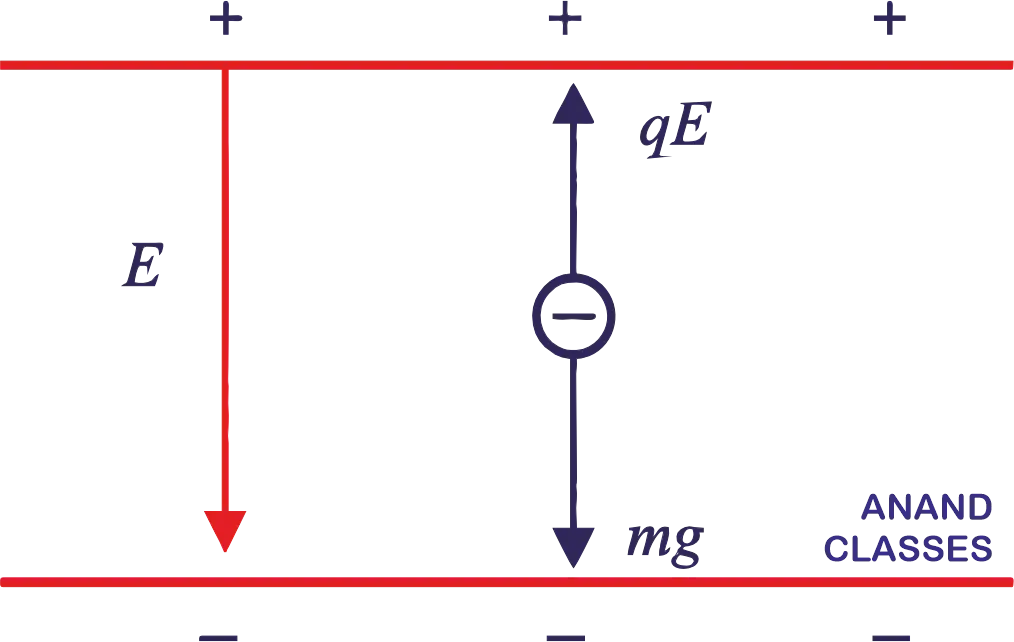
When the drop is held stationary,

Upward force on oil drop due to electric field = Weight of oil drop

qE = mg

$q cdot dfrac{V}{d} = mg$

$V = dfrac{mg cdot d}{q} = dfrac{3 times 10^{-16} times 10 times 5 times 10^{-3}}{10 times 1.6 times 10^{-19}} = 9.375text{ V}$

---

How many electrons should be removed from a coin of mass 1.6 g, so that it may just float in an electric field of intensity 10⁹ NC^-1, directed upward?

Solution. Given m = 1.6 g = 1.6 × 10^-3 kg, E = 10⁹ NC^-1. Let n be the number of electrons removed from the coin. Then charge on the coin, q = +ne.

When the coin just floats,

Upward force of electric field = Weight of coin

qE = mg

(ne)E = mg

$n = dfrac{mg}{eE} = dfrac{1.6 times 10^{-3} times 9.8}{1.6 times 10^{-19} times 10^9} = 9.8 times 10^7$

---

A pendulum of mass 80 milligram carrying a charge of 2 × 10^-8 C is at rest in a horizontal uniform electric field of 2 × 10⁴ Vm^-1. Find the tension in the thread of the pendulum and the angle it makes with the vertical. [IIT 1979]

Solution. Given m = 80 mg = 80 × 10^-6 kg, q = 2 × 10^-8 C, E = 2 × 10⁴ Vm^-1.

Let T be the tension in the thread and θ be the angle it makes with vertical.

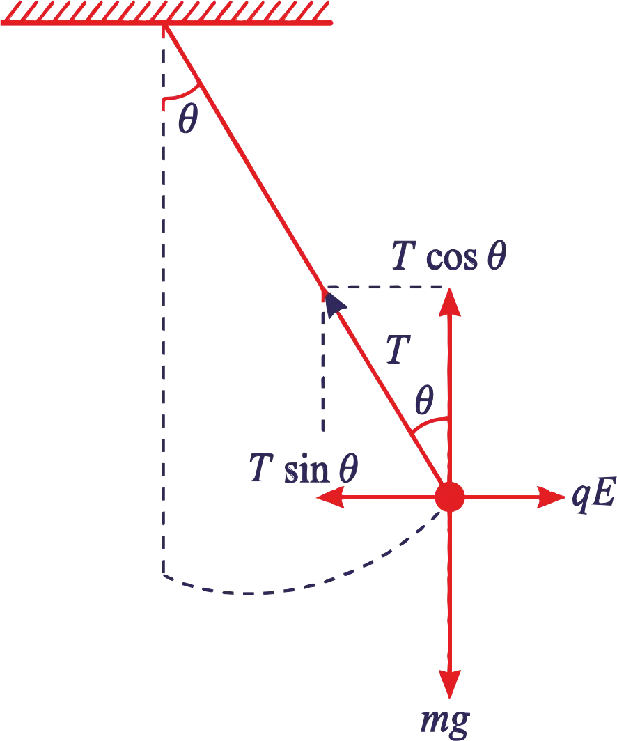
When the bob is in equilibrium,

T sinθ = qE

T cosθ = mg

Also,

$tan theta = dfrac{T sin theta}{T cos theta} = dfrac{qE}{mg} = dfrac{2 times 10^{-8} times 2 times 10^4}{80 times 10^{-6} times 9.8} = 0.51$

θ = 27°

$T = dfrac{qE}{sin theta} = dfrac{2 times 10^{-8} times 2 times 10^4}{sin 27^circ} = 8.81 times 10^{-4}text{ N}$

---

An electron moves a distance of 6 cm when accelerated from rest by an electric field of strength 2 × 10⁴ NC^-1. Calculate the time of travel. The mass and charge of electron are 9 × 10^-31 kg and 1.6 × 10^-19 C respectively.

Solution. Force exerted on the electron by the electric field,

F = eE

$therefore text{Acceleration, } a = dfrac{F}{m}$

$a = dfrac{eE}{m} = dfrac{1.6 times 10^{-19} times 2 times 10^4}{9 times 10^{-31}} = 0.35 times 10^{16}text{ ms}^{-2}$

Now u = 0, s = 6.0 cm = 0.06 m, a = 0.35 × 10¹⁶ ms^-2, now

$s = ut + dfrac{1}{2}at^2$

$0.06 = 0 + dfrac{1}{2} times 0.35 times 10^{16} times t^2$

$t = sqrt{dfrac{0.06 times 2}{0.35 times 10^{16}}} = 0.585 times 10^{-8}text{ s}$

---

An electron falls through a distance of 1.5 cm in a uniform electric field of magnitude 2.0 × 10⁴ NC^-1. The direction of the field is reversed keeping its magnitude unchanged and a proton falls through the same distance. Compute the time of fall in each case. Contrast the situation (a) with that of ‘free fall under gravity’. [NCERT]

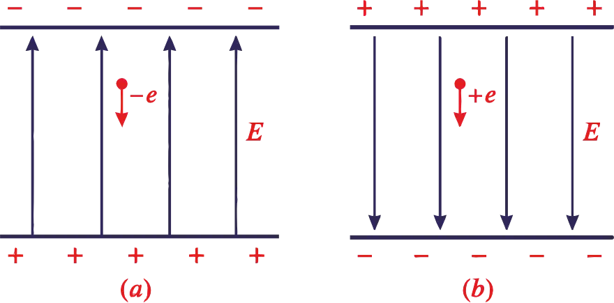
Solution.

(a) The upward field exerts a downward force eE on the electron.

$therefore text{Acceleration of the electron, } a_e = dfrac{eE}{m_e}$

$text{As } u = 0, quad s = ut + dfrac{1}{2}at^2 = dfrac{1}{2}at^2,$

therefore time of fall of the electron is,

$t_e = sqrt{dfrac{2s}{a_e}} = sqrt{dfrac{2s m_e}{eE}}$

$t_e = sqrt{dfrac{2 times 1.5 times 10^{-2} times 9.1 times 10^{-31}}{1.6 times 10^{-19} times 2.0 times 10^4}} = 2.9 times 10^{-9}text{ s}$

(b) The downward field exerts a downward force eE on the proton.

$therefore a_p = dfrac{eE}{m_p}$

Time of fall of the proton is,

$t_p = sqrt{dfrac{2s}{a_p}} = sqrt{dfrac{2s m_p}{eE}}$

$t_p = sqrt{dfrac{2 times 1.5 times 10^{-2} times 1.67 times 10^{-27}}{1.6 times 10^{-19} times 2.0 times 10^4}} = 1.25 times 10^{-7}text{ s}$

Thus the heavier particle takes a greater time to fall through the same distance. This is in contrast to the situation of ‘free fall under gravity’ where the time of fall is independent of the mass of the body. Here the acceleration due to gravity ‘g‘, being negligibly small, has been ignored.

---

An electron is liberated from the lower of the two large parallel metal plates separated by a distance of 20 mm. The upper plate has a potential of +2400 V relative to the lower plate. How long does the electron take to reach the upper plate? Take e/m of electrons 1.8 × 10¹¹ C kg^-1.

Solution. Here V = 2400 V, d = 20 mm = 0.02 m, e/m = 1.8 × 10¹¹ C kg^-1

Upward force on the electron exerted by electric field is

$F = eE = dfrac{eV}{d}$

$therefore text{Acceleration, } a = dfrac{F}{m} = dfrac{eV}{md}$

$a = dfrac{1.8 times 10^{11} times 2400}{0.02}text{ ms}^{-2} = 2.16 times 10^{16}text{ ms}^{-2}$

Using, $s = dfrac{1}{2}at^2$, we get

$t = sqrt{dfrac{2s}{a}} = sqrt{dfrac{2d}{a}} = sqrt{dfrac{2 times 0.02}{2.16 times 10^{16}}}text{ s} = 1.4 times 10^{-9}text{ s}$

---

A stream of electrons moving with a velocity of 3 × 10⁷ ms^-1 is deflected by 2 mm in traversing a distance of 0.1 m in a uniform electric field of strength 18 V cm^-1. Determine e/m of electrons.

Solution. Here v₀ = 3 × 10⁷ ms^-1, y = 2 mm = 2 × 10^-3 m,

x = 0.1 m, E = 18 V cm^-1 = 1800 V m^-1

$ma = eE quad text{or} quad a = dfrac{eE}{m} quad text{and} quad t = dfrac{x}{v_0}$

$y = dfrac{1}{2}at^2 = dfrac{1}{2}dfrac{eE}{m} dfrac{x^2}{v_0^2}$

$dfrac{e}{m} = dfrac{2y v_0^2}{Ex^2} = dfrac{2 times 2 times 10^{-3} times 9 times 10^{14}}{1800 times (0.1)^2} = 2 times 10^{11}text{ C kg}^{-1}$

---

An electric field E is set up between the two parallel plates of a capacitor as shown in Figure. An electron enters the field symmetrically between the plates with a speed v₀. The length of each plate is l. Find the angle of deviation of the path of the electron as it comes out of the field.

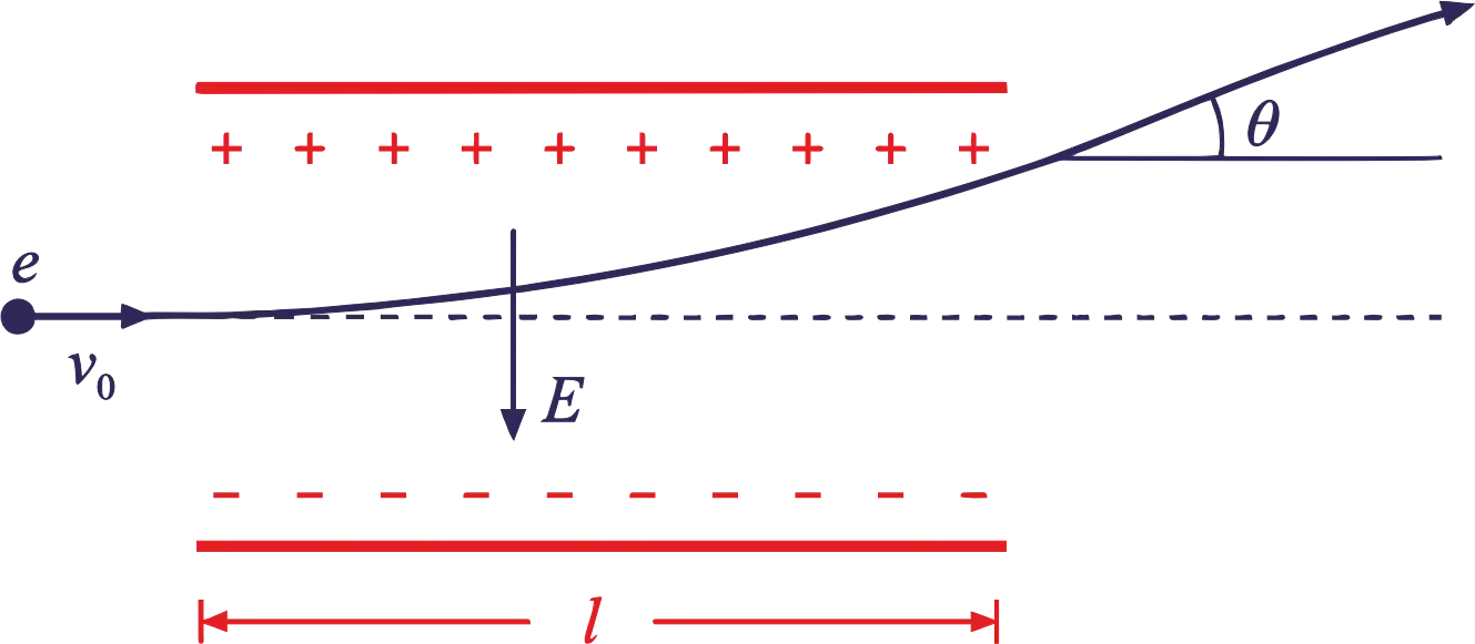
Solution. Acceleration of the electron in the upward direction,

$a = dfrac{eE}{m}$

Time taken to cross the field, $t = dfrac{l}{v_0}$

Upward component of electron velocity on emerging from field region,

$v_y = at = dfrac{eEl}{mv_0}$

Horizontal component remains same, v_x = v₀

If θ is the angle of deviation of the path of the electron, then

$tan theta = dfrac{v_y}{v_x} = dfrac{eEl}{mv_0^2} quad text{or} quad theta = tan^{-1} dfrac{eEl}{mv_0^2}$

---

A charged particle, of charge 2 μC and mass 10 milligram, moving with a velocity of 1000 m/s enters a uniform electric field of strength 10³ NC^-1 directed perpendicular to its direction of motion. Find the velocity and displacement, of the particle after 10 seconds.

Solution. The velocity of the particle, normal to the direction of field,

v_x = 1000 ms^-1 is constant

The velocity of the particle, along the direction of field, after 10 seconds, is given by

$v_y = u_y + a_y t$

$v_y = 0 + dfrac{qE_y}{m} t = dfrac{2 times 10^{-6} times 10^3 times 10}{10 times 10^{-6}} = 2000text{ ms}^{-1}$

The net velocity after 10 seconds,

$v = sqrt{v_x^2 + v_y^2} = sqrt{(1000)^2 + (2000)^2} = 1000sqrt{5}text{ ms}^{-1}$

Displacement, along the x-axis, after 10 seconds,

x = 1000 × 10 m = 10000 m

Displacement along y-axis (in the direction of field) after 10 seconds,

$y = u_y t + dfrac{1}{2} a_y t^2 = (0)t + dfrac{1}{2} dfrac{qE_y}{m} t^2$

$y = dfrac{1}{2} times dfrac{2 times 10^{-6} times 10^3}{10 times 10^{-6}} times (10)^2$

y = 10000 m

Net displacement,

$= sqrt{x^2 + y^2} = sqrt{(10000)^2 + (10000)^2} = 10000sqrt{2}text{ m}$

---

An oil drop of 12 excess electrons is held stationary under a constant electric field of 2.55 × 10⁴ NC^-1 in Millikan’s oil drop experiment. The density of the oil is 1.26 g cm^-3. Estimate the radius of the drop. (g = 9.81 ms^-2 ; e = 1.6 × 10^-19 C)

Solution. Given, n = 12, E = 2.55 × 10⁴ NC^-1,

ρ = 1.26 g cm^-3 = 1.26 × 10³ kg m^-3, r = ?

Force due to electric field = qE = (ne)E

Weight of droplet = mg = (ρ × 4/3πr³)g

As the droplet is stationary, therefore

Weight of droplet = Force due to electric field

$dfrac{4}{3}pi r^3 rho g = n e E quad ;$

$r^3 = dfrac{3 E n e}{4 pi rho g}$

$r^3 = dfrac{3 times 2.55 times 10^4 times 12 times 1.6 times 10^{-19}}{4 times 3.14 times 1.26 times 10^3 times 9.81}$

$r^3 = 0.94 times 10^{-18}$

$therefore r = (0.94 times 10^{-18})^{1/3} = 9.81 times 10^{-7}text{ m}$

---

A small sphere of mass 1 g carries a charge of +6 μC. The sphere is suspended by a string in an electric field of 400 NC^-1 acting downwards. Calculate tension in the string. What will be the tension if charge on the sphere were -6 μC ?

Solution. Given, m = 1 g = 10^-3 kg,

q = +6 μC = +6 × 10^-6 C, E = 400 NC^-1, downwards

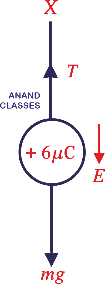
The vertical forces according to the Figure shown are as follows :

T = F_e + mg = qE + mg

T = 6 × 10^-6 × 400 + 10^-3 × 9.8

T = 1.22 × 10^-2 N

However, when q = -6 μC, force due to electric field is upwards. Therefore

T + F_e = mg

T = mg – F_e

T = 9.8 × 10^-3 – 24 × 10^-4

T = 74 × 10^-4 N

---

A particle of mass 10^-3 kg and charge 5 μC is thrown at a speed 20 ms^-1 against a uniform electric field of strength 2 × 10⁵ NC^-1. How much distance will it travel before coming to rest momentarily?

Solution

Given: m = 10^-3 kg, q = 5 μC = 5 × 10^-6 C, u = 20 ms^-1, E = 2 × 10⁵ NC^-1

The force on the charged particle is :

F = qE = (5 × 10^-6 C) × (2 × 10⁵ NC^-1) = 1 N

Since the particle is thrown against the electric field, the force acts as a retarding force. The acceleration of the particle is :

$a = -dfrac{F}{m} = -dfrac{1text{ N}}{10^{-3}text{ kg}} = -10^3text{ m s}^{-2}$

The distance traveled (S) by particle before coming to rest (v = 0) is :

Using the equation of motion $v^2 – u^2 = 2aS$ :

$S = dfrac{v^2 – u^2}{2a}$

$S = dfrac{0^2 – (20)^2}{2 times (-10^3)} = dfrac{-400}{-2000} = 0.2text{ m}$

The particle will travel 0.2 m before coming to rest momentarily.

---

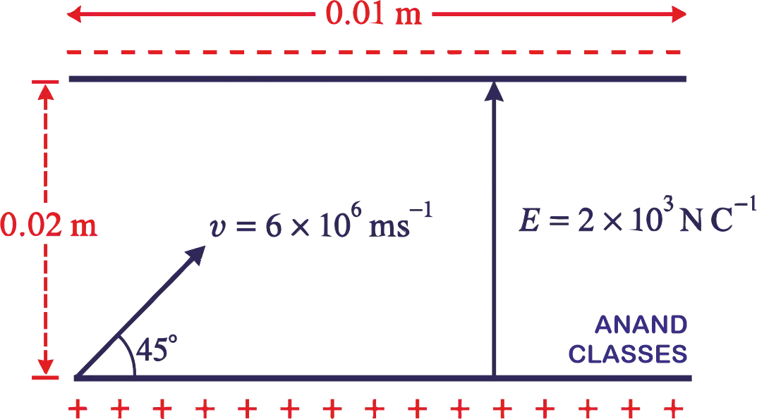
A uniform electric field of strength 2 × 10³ NC^-1 is established between two parallel plates of length 0.1 m held horizontally at a distance 0.02 m apart. An electron is projected at a speed of 6 × 10⁶ ms^-1 making an angle 45° as shown in Figure. The field is directed vertically upwards. Will the electron strike either plate? If it strikes the plate, where does it do so?

Solution :

The initial speed of the electron v = 6 × 10⁶ ms^-1 can be resolved into two perpendicular components:

Horizontal Component (v_x) : v_x = v cos 45° = 6 × 10⁶ × 0.707 = 4.24 × 10⁶ ms^-1 along horizontal. Since there is no force acting on the electron in the horizontal direction, v_x remains unchanged.

Vertical Component (v_y) : v_y = v sin 45° = 6 × 10⁶ × 0.707 = 4.24 × 10⁶ ms^-1 along vertical.

Since the electric field (E) is directed vertically upwards and an electron carries a negative charge (q), the electron experiences an electric force in the downward direction (opposite to the field).

Given q = 1.6 × 10^-19 C, m = 9.1 × 10^-31 kg, E = 2 × 10³ NC^-1

Force on electron, F = qE (downwards)

Downward acceleration $a = dfrac{F}{m} = dfrac{qE}{m}$

$a = dfrac{1.6 times 10^{-19} times 2 times 10^3}{9.1 times 10^{-31}}$

$a = 3.516 times 10^{14}text{ m s}^{-2} quad text{(downwards)}$

For motion along the vertical direction :

Initial vertical velocity: uᵧ = 4.24 × 10⁶ m s⁻¹
Vertical acceleration: aᵧ = −3.516 × 10¹⁴ m s⁻²
Vertical displacement to reach upper plate: S = 0.02 m

Using the relation $S = u_y t + dfrac{1}{2}a_y t^2$ :

$0.02 = (4.24 times 10^6) t + dfrac{1}{2} (-3.516 times 10^{14}) t^2$

$1.758 times 10^{14} t^2 – 4.24 times 10^6 t + 0.02 = 0$

t = 6.4 × 10^-9 seconds

Since t has a real, positive value, the electron will strike the upper plate.

Suppose the electron strikes the upper plate at a horizontal distance x from the point of projection:

x = vₓ × t
x = (4.24 × 10⁶ m s⁻¹) × (6.4 × 10⁻⁹ s)

x = 2.71 × 10⁻² m = 2.71 cm

---

Electric Field Intensity due to a Point Charge

Consider a point charge +Q is placed at the origin O of the co-ordinate frame. Let P be the point, where electric field due to the point charge +Q is to be determined. Let OP = r₀ be the position vector of the point P.

To find electric field at point P, place a vanishingly small positive test charge q₀ at point P. According to Coulomb’s law, force on the test charge q₀ due to charge Q is given by

$vec{F} = dfrac{1}{4pivarepsilon_0} dfrac{Q q_0}{r_0^2} hat{r}_0$

where $hat{r}_0$ is unit vector directed from Q towards q₀.

As $vec{E} = dfrac{vec{F}}{q_0}$

$quad therefore quad vec{E} = dfrac{1}{4pivarepsilon_0} dfrac{Q}{r_0^2} hat{r}_0$

From the above expression for electric field, it follows that electric field is spherically symmetric as seen from the charge Q and its magnitude decreases inversely as the square of the distance from the charge. Such a field is called spherically symmetric or radial field, i.e., a field which looks the same in all directions when seen from the point charge.

Now, suppose the point charge +Q is situated at A, where $vec{OA} = vec{r}_i$.

We have to calculate electric field intensity ($vec{E}$) at P, where $vec{OP} = vec{r}_0$ and $vec{AP} = vec{r}_{i0}$

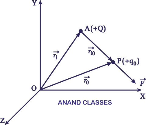
According to Coulomb’s law, force on a small test charge +q₀ at P due to source charge Q at A is

$vec{F} = dfrac{1}{4pivarepsilon_0} dfrac{Q q_0}{AP^2}$

$vec{F} = dfrac{1}{4pivarepsilon_0} dfrac{Q q_0}{r_{i0}^2} hat{r}_{i0} = dfrac{1}{4pivarepsilon_0} dfrac{Q q_0}{r_{i0}^3} vec{r}_{i0}$

$vec{F} = dfrac{1}{4pivarepsilon_0} dfrac{Q q_0}{vert{}vec{r}_0 – vec{r}_ivert{}^3} (vec{r}_0 – vec{r}_i)$

where $vec{r}_0 – vec{r}_i = vec{r}_{i0} = vec{AP}$

As $vec{E} = dfrac{vec{F}}{q_0}$

$therefore quad vec{E} = dfrac{1}{4pivarepsilon_0} dfrac{Q}{vert{}vec{r}_0 – vec{r}_ivert{}^3} (vec{r}_0 – vec{r}_i)$

The direction of above electric field is along $vec{AP}$.

---

Representation of Electric Field due to a Point Charge

Let us represent the electric field due to a positive charge by associating a vector (in order to represent magnitude and direction). The magnitude and direction of the electric field at various points may be represented by arrows of suitable lengths. The points, where the electric field has large magnitude, longer arrows may be used and at the points, where the field has small magnitude, smaller arrows may be used. To be accurate, the lengths of the arrows will vary inversely as the square of the distance of the observation point from the charge.

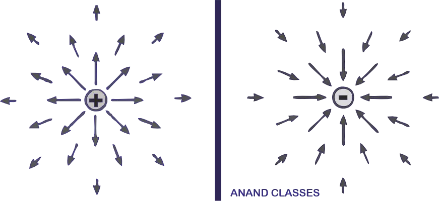
Further, in case a positive charge, the arrows will point away from the charge, and will point into the charge, in case it is a negative charge. The above Figure represents the electric field due to a positive point charge, and the electric field due to a negative point charge.

Key Point
The electric field due to a point charge is spherically symmetric about the charge.

---

Electric Field Intensity at any point due to Group of Discrete Point Charges

The resultant (or net) electric field intensity at a point due to a group of discrete point charges can be found by applying superposition principle.

The electric field intensity at any point due to a group of point charges is equal to the vector sum of the electric field intensities due to individual charges at the same point.

Consider a system of N point charges q₁, q₂, ……, q_N having position vectors $vec{r}_1, vec{r}_2, dots, vec{r}_N$ with respect to the origin O. We want to calculate the electric field at a point P whose position vector is $vec{r}$.

According to Coulomb’s law, the force on test charge q₀ due to charge q₁ is

$vec{F}_1 = dfrac{1}{4pivarepsilon_0} dfrac{q_1 q_0}{r_{1P}^2} hat{r}_{1P}$

where $hat{r}_{1P}$ is a unit vector in the direction from q₁ to P and r_1P is the distance between q₁ and P. Hence the electric field at point P due to charge q₁ is

$vec{E}_1 = dfrac{vec{F}_1}{q_0} = dfrac{1}{4pivarepsilon_0} dfrac{q_1}{r_{1P}^2} hat{r}_{1P}$

Similarly, electric field at P due to charge q₂ is

$vec{E}_2 = dfrac{1}{4pivarepsilon_0} dfrac{q_2}{r_{2P}^2} hat{r}_{2P}$

According to the principle of superposition of electric fields, the electric field at any point due to a group of charges is equal to the vector sum of the electric fields produced by each charge individually at that point, when all other charges are assumed to be absent.

Hence, the electric field at point P due to the system of N charges is

$vec{E} = vec{E}_1 + vec{E}_2 + dots + vec{E}_N$

$= dfrac{1}{4pivarepsilon_0} left[ dfrac{q_1}{r_{1P}^2} hat{r}_{1P} + dfrac{q_2}{r_{2P}^2} hat{r}_{2P} + dots + dfrac{q_N}{r_{NP}^2} hat{r}_{NP} right]$

$text{or} quad vec{E} = dfrac{1}{4pivarepsilon_0} sum_{i=1}^{N} dfrac{q_i}{r_{iP}^2} hat{r}_{iP}$

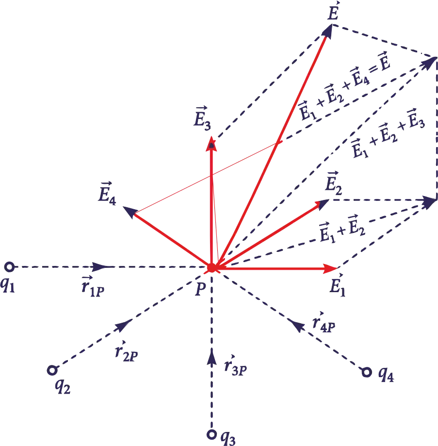
In terms of position vectors, we can write

$vec{E} = dfrac{1}{4pivarepsilon_0} sum_{i=1}^{N} dfrac{q_i}{vert{}vec{r} – vec{r}_ivert{}^2} cdot dfrac{vec{r} – vec{r}_i}{vert{}vec{r} – vec{r}_ivert{}}$

$text{or} quad vec{E} = dfrac{1}{4pivarepsilon_0} sum_{i=1}^{N} dfrac{q_i}{vert{}vec{r} – vec{r}_ivert{}^3} (vec{r} – vec{r}_i).$

Note that $vec{E}$ is a vector quantity that varies from one point to another point in space. Its value depends on the positions of the source charges. The direction of $vec{E}$ due to a group of discrete charges is determined using polygon law of vectors.

Conceptual Question Two point charges of 3 μC each are 100 cm apart At what point on the line joining the charges will the electric field intensity be zero ?
Electric filed intensity be zero at the centre of the two charges.

---

Electric Field Intensity due to Continuous Charge Distribution

In practice, we deal with charges much greater in magnitude than the charge on an electron, so we can ignore the quantum nature of charges and imagine that the charge is spread in a region in a continuous manner. Such a charge distribution is known as a continuous charge distribution.

Consider a point charge q₀ lying near a region of continuous charge distribution. This continuous charge distribution can be imagined to consist of a large number of small charges dq. According to Coulomb’s law, the force on point charge q₀ due to small charge dq is

$dvec{F} = dfrac{1}{4pivarepsilon_0} dfrac{q_0 , dq}{r^2} hat{r}$

where $hat{r} = dfrac{vec{r}}{r}$, is a unit vector pointing from the small charge dq towards the point charge q₀.

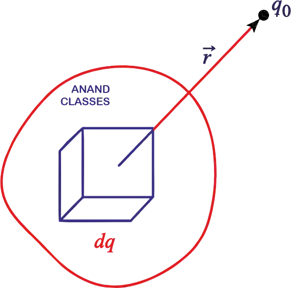
By the principle of superposition, the total force on charge q₀ will be the vector sum of the forces exerted by all such small charges and is given by

$vec{F} = int dvec{F} = int dfrac{1}{4pivarepsilon_0} cdot dfrac{q_0 , dq}{r^2} hat{r}$

or

$vec{F} = dfrac{q_0}{4pivarepsilon_0} int dfrac{dq}{r^2} hat{r}$

Therefore electric field intensity at location $vec{r}$ is

$vec{E} = dfrac{1}{4pivarepsilon_0} int dfrac{dq}{r^2} hat{r}$

There are three types of continuous charge distributions which are discuss as follows :

(a) Volume charge distribution

It is a charge distribution spread over a three dimensional volume or region V of space, as shown in Figure. We define the volume charge density at any point in this volume as the charge contained per unit volume at that point, i.e.,

$rho = dfrac{dq}{dV}$

The SI unit for ρ is coulomb per cubic metre (C m^-3).

For example, if a charge q is distributed over the entire volume of a sphere of radius R, then its volume charge density is

$rho = dfrac{q}{dfrac{4}{3} pi R^3} text{ C m}^{-3}$

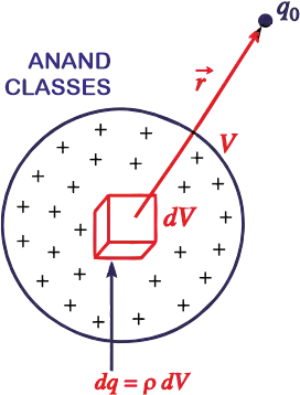
The charge contained in small volume dV is

dq = ρ dV

Total electrostatic force exerted on charge q₀ due to the entire volume V is given by

$vec{F}_V = dfrac{q_0}{4pivarepsilon_0} int_V dfrac{dq}{r^2} hat{r} = dfrac{q_0}{4pivarepsilon_0} int_V dfrac{rho}{r^2} , dV , hat{r}$

Electric field due to the volume charge distribution at the location of charge q₀ is

$vec{E}_V = dfrac{vec{F}_V}{q_0} = dfrac{1}{4pivarepsilon_0} int_V dfrac{rho}{r^2} , dV , hat{r}$

(b) Surface charge distribution

It is a charge distribution spread over a two-dimensional surface S in space, as shown in Figure. We define the surface charge density at any point on this surface as the charge per unit area at that point, i.e.,

$sigma = dfrac{dq}{dS}$

The SI unit for σ is coulomb per square metre (C m^-2).

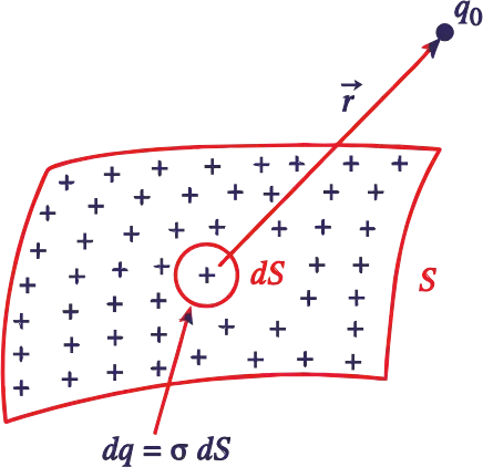
For example, if a charge q is uniformly distributed over the surface of a spherical conductor of radius R, then its surface charge density is

$sigma = dfrac{q}{4pi R^2} text{ C m}^{-2}$

The charge contained in small area dS is

dq = σ dS

Total electrostatic force exerted on charge q₀ due to the entire surface S is given by

$vec{F}_S = dfrac{q_0}{4pivarepsilon_0} int_S dfrac{dq}{r^2} hat{r} = dfrac{q_0}{4pivarepsilon_0} int_S dfrac{sigma}{r^2} , dS , hat{r}$

Electric field due to the surface charge distribution at the location of charge q₀ is

$vec{E}_S = dfrac{vec{F}_S}{q_0} = dfrac{1}{4pivarepsilon_0} int_S dfrac{sigma}{r^2} , dS , hat{r}$

(c) Line charge distribution

It is a charge distribution along a one-dimensional curve or line L in space, as shown in Figure. We define the line charge density at any point on this line as the charge per unit length of the line at that point, i.e.,

$lambda = dfrac{dq}{dL}$

The SI unit for λ is coulomb per metre (C m^-1).

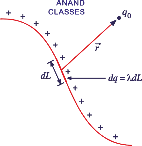
For example, if a charge q is uniformly distributed over a ring of radius R, then its linear charge density is

$lambda = dfrac{q}{2pi R} text{ C m}^{-1}$

The charge contained in small length dL is

dq = λ dL

Total electrostatic force exerted on charge q₀ due to the entire length L is given by

$vec{F}_L = dfrac{q_0}{4pivarepsilon_0} int_L dfrac{dq}{r^2} hat{r} = dfrac{q_0}{4pivarepsilon_0} int_L dfrac{lambda}{r^2} , dL , hat{r}$

Electric field due to the line charge distribution at the location of charge q₀ is

$vec{E}_L = dfrac{vec{F}_L}{q_0} = dfrac{1}{4pivarepsilon_0} int_L dfrac{lambda}{r^2} , dL , hat{r}$

The total electric field due to a continuous charge distribution is given by

$vec{E}_{text{continous}} = vec{E}_V + vec{E}_S + vec{E}_L$

or

$vec{E}_{text{continous}} = dfrac{1}{4pivarepsilon_0} left[ int_V dfrac{rho}{r^2} , dV , hat{r} + int_S dfrac{sigma}{r^2} , dS , hat{r} + int_L dfrac{lambda}{r^2} , dL , hat{r} right]$

General Charge Distribution

A general charge distribution consists of continuous as well as discrete charges. Hence total electric field due to a general charge distribution at the location of charge q₀ is given by

$vec{E}_{text{total}} = vec{E}_{text{discrete}} + vec{E}_{text{continous}}$

or

$vec{E}_{text{total}} = dfrac{1}{4pivarepsilon_0} left[ sum_{i=1}^{N} dfrac{q_i}{r_i^2} hat{r}_i + int_V dfrac{rho}{r^2} , dV , hat{r} + int_S dfrac{sigma}{r^2} , dS , hat{r} + int_L dfrac{lambda}{r^2} , dL , hat{r} right]$

---

Rectangular Components of Electric Field Intensity due to a Point Charge

Consider a point charge +q is held at O, the origin of co-ordinate system. We are to find the rectangular components of electric field intensity ($vec{E}$) at any point P(x, y, z), where

$vec{OP} = vec{r} = hat{i}x + hat{j}y + hat{k}z$

$r = vert{}vec{r}vert{} = sqrt{x^2 + y^2 + z^2}$

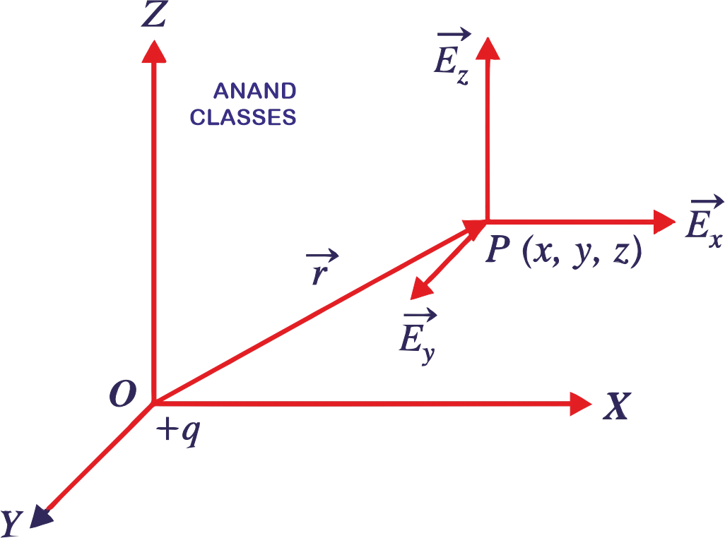
Electric Field Intensity at P due to charge q at O i.e.

$vec{E} = dfrac{1}{4pivarepsilon_0} dfrac{q}{r^2} hat{r}$

$vec{E} = dfrac{q}{4pivarepsilon_0 r^3} vec{r} = dfrac{q(hat{i}x + hat{j}y + hat{k}z)}{4pivarepsilon_0 (x^2 + y^2 + z^2)^{3/2}}$

If $vec{E}_x, vec{E}_y, vec{E}_z$ are the components of $vec{E}$ along the three co-ordinate axes, then

$vec{E} = vec{E}_x + vec{E}_y + vec{E}_z quad text{or} quad vec{E} = hat{i}E_x + hat{j}E_y + hat{k}E_z$

Hence, rectangular components of electric field intensity are as follows :

$E_x = dfrac{q x}{4pivarepsilon_0 (x^2 + y^2 + z^2)^{3/2}}$

$E_y = dfrac{q y}{4pivarepsilon_0 (x^2 + y^2 + z^2)^{3/2}}$

$E_z = dfrac{q z}{4pivarepsilon_0 (x^2 + y^2 + z^2)^{3/2}}$

We find from above equations that as seen from O, the position of point charge +q, the electric field is spherically symmetric, i.e., at x = y = z ; E_x = E_y = E_z, i.e., at equal distances from the charge, field intensity is equal. Further, electric intensity at any point varies inversely as the square of the distance of the point from the charge.

---

Solved Numerical Problems on Electric Field and Electric Field Intensity due to Point Charge, Group of Charges and Continuous Charge Distribution for Class 12 Physics, JEE and NEET

The section covers solved numerical problems on electric field and electric field intensity due to a point charge, a group of discrete charges, and continuous charge distributions. The problems include different charge configurations and applications of the principle of superposition, providing practice in calculating electric field magnitude, direction, and resultant electric field for Class 12 Physics, JEE and NEET exams.

Assuming that the charge on an atom is distributed uniformly in a sphere of radius 10^-10 m, what will be the electric field at the surface of the gold atom? For gold, Z = 79.

Solution:

The charge may be assumed to be concentrated at the centre of the sphere of radius 10^-10 m.

Take r = 10^-10 m, q = Ze = 79 × 1.6 × 10^-19 C

$E = dfrac{1}{4pivarepsilon_0} cdot dfrac{q}{r^2}$

$E = dfrac{9 times 10^9 times 79 times 1.6 times 10^{-19}}{(10^{-10})^2}$

$E = 1.138 times 10^{13}text{ NC}^{-1}$

---

Two point charges of 2.0 × 10^-7 C and 1.0 × 10^-7 C are 1.0 cm apart. What is the magnitude of the field produced by either charge at the site of the other?

Solution: Here: q₁ = 2.0 × 10^-7 C, q₂ = 1.0 × 10^-7 C, r = 1.0 cm = 0.01 m

Electric field due to q₁ at the site of q₂ :

$E_1 = dfrac{1}{4pivarepsilon_0} cdot dfrac{q_1}{r^2}$

$E_1 = dfrac{9 times 10^9 times 2.0 times 10^{-7}}{(0.01)^2} = 1.8 times 10^7text{ NC}^{-1}$

Electric field due to q₂ at the site of q₁ :

$E_2 = dfrac{1}{4pivarepsilon_0} cdot dfrac{q_2}{r^2}$

$E_2 = dfrac{9 times 10^9 times 1.0 times 10^{-7}}{(0.01)^2} = 9 times 10^6text{ NC}^{-1}$

---

Two point charges of +5 × 10^-19 C and +20 × 10^-19 C are separated by a distance of 2 m. Find the point on the line joining them at which electric field intensity is zero.

Solution.

Let q₁ = +5 × 10^-19 C and q₂ = +20 × 10^-19 C.

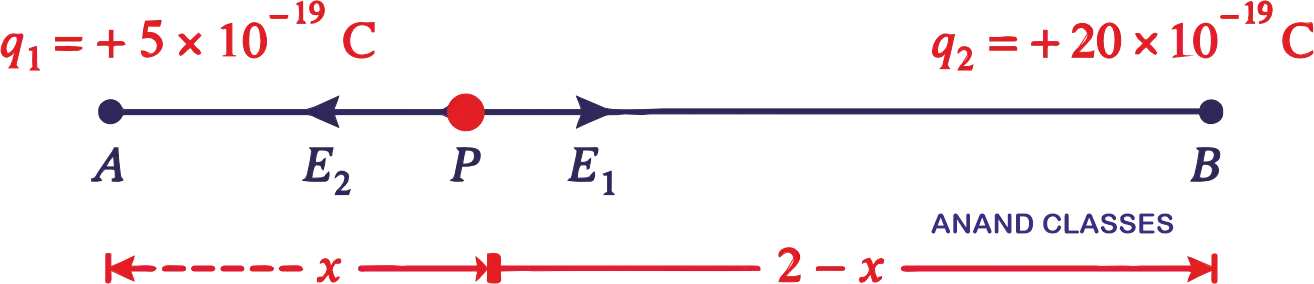
The electric field at point P will be zero if

E₁ = E₂

$dfrac{1}{4pivarepsilon_0} cdot dfrac{5 times 10^{-19}}{x^2} = dfrac{1}{4pivarepsilon_0} cdot dfrac{20 times 10^{-19}}{(2 – x)^2}$

$text{or } 4x^2 = (2 – x)^2 quad text{or} quad 2x = pm (2 – x)$

$text{or } x = 2/3text{ m} quad text{or} quad -2text{ m}$

At x = -2 m i.e., at 2 m left of q₁, electric fields due to both charges will be in same direction. So x = -2 m is not a possible solution.

Hence electric field will be zero at 2/3 m to the right of q₁.

---

Two point charges of +16 μC and -9 μC are placed 8 cm apart in air. Determine the position of the point at which the resultant field is zero.

Solution. Let P be the point at distance x cm from A, where the net field is zero.

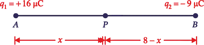
q₁ = +16 μC, q₂ = -9 μC

At point P, $vec{E}_1 + vec{E}_2 = 0$

$dfrac{k times 16 times 10^{-6}}{(x times 10^{-2})^2} + dfrac{k times (-9) times 10^{-6}}{[(8 – x) times 10^{-2}]^2} = 0$

$dfrac{16}{x^2} = dfrac{9}{(8 – x)^2}$

$dfrac{4}{x} = pm dfrac{3}{8 – x}$

$x = -dfrac{32}{7}text{ cm}, 32text{ cm}$

At $x = -dfrac{32}{7}text{ cm}$, both $vec{E}_1$ and $vec{E}_2$ will be in the same direction, therefore, net electric field cannot be zero.

Hence, x = 32 cm i.e., electric field is zero at a point 24 cm to the right of -9 μC charge.

---

Two point charges q₁ = +0.2 C and q₂ = +0.4 C are placed 0.1 m apart. Calculate the electric field at:
(a) the midpoint between the charges.
(b) a point on the line joining q₁ and q₂ such that it is 0.05 m away from q₂ and 0.15 m away from q₁.

Solution. (a) Let O be the midpoint between the two charges.

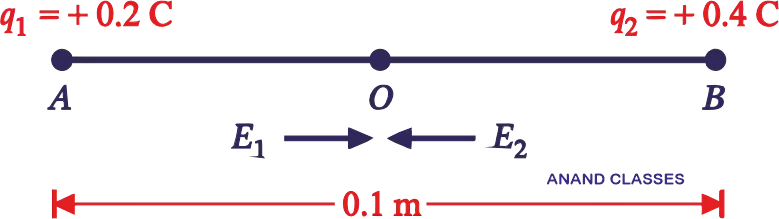
Electric field at O due to q₁ :

$E_1 = dfrac{k q_1}{r_1^2} = dfrac{9 times 10^9 times 0.2}{(0.05)^2}$

E₁ = 7.2 × 10¹¹ NC^-1, acting along AO

Electric field at O due to q₂ :

$E_2 = dfrac{k q_2}{r_2^2} = dfrac{9 times 10^9 times 0.4}{(0.05)^2}$

E₂ = 14.4 × 10¹¹ NC^-1, acting along BO

Net field at O = E₂ – E₁ = 7.2 × 10¹¹ NC^-1, acting along BO.

(b) Electric field at P due to q₁ :

$E_1 = dfrac{k q_1}{r_1^2} = dfrac{9 times 10^9 times 0.2}{(0.15)^2}, text{ acting along } AP$

Electric field at P due to q₂ :

$E_2 = dfrac{k q_2}{r_2^2} = dfrac{9 times 10^9 times 0.4}{(0.05)^2}, text{ acting along } BP$

Net electric field at point P is

$E = E_1 + E_2 = 9 times 10^9 left[ dfrac{0.2}{(0.15)^2} + dfrac{0.4}{(0.05)^2} right]$

$E = 1.52 times 10^{12}text{ NC}^{-1}, text{ acting along } AP$

---

Two point charges q₁ and q₂ of 10^-8 C and -10^-8 C respectively are placed 0.1 m apart. Calculate the electric fields at points A, B and C shown in Figure, [NCERT]

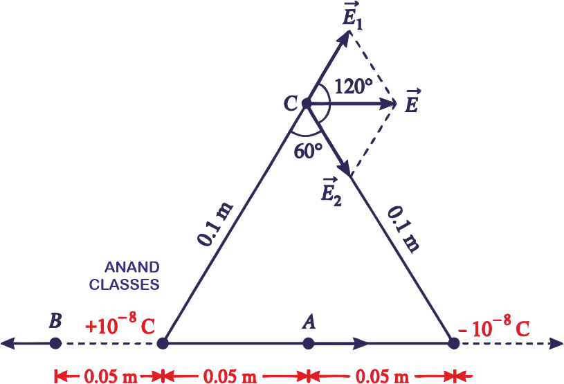
Solution. The electric field vector $vec{E}_1$ at A due to the positive charge q₁ points towards the right and it has a magnitude,

$E_1 = dfrac{k q_1}{r^2} = dfrac{9 times 10^9 times 10^{-8}}{(0.05)^2}text{ NC}^{-1} = 3.6 times 10^4text{ NC}^{-1}$

The electric field vector $vec{E}_2$ at A due to the negative charge q₂ points towards the right and it has a magnitude,

$E_2 = dfrac{9 times 10^9 times 10^{-8}}{(0.05)^2}text{ NC}^{-1} = 3.6 times 10^4text{ NC}^{-1}$

Magnitude of the total electric field at A

$E_a = E_1 + E_2 = 3.6 times 10^4 + 3.6 times 10^4$

$E_a = 7.2 times 10^4text{ NC}^{-1}$

$vec{E}_a$ is directed towards the right.

The electric field vector $vec{E}_1$ at B due to the positive charge q₁ points towards the left and it has a magnitude,

$E_1 = dfrac{9 times 10^9 times 10^{-8}}{(0.05)^2}text{ NC}^{-1}$

$E_1 = 3.6 times 10^4text{ NC}^{-1}$

The electric field vector $vec{E}_2$ at B due to the negative charge q₂ points towards the right and it has a magnitude,

$E_2 = dfrac{9 times 10^9 times 10^{-8}}{(0.15)^2}text{ NC}^{-1} = 4 times 10^3text{ NC}^{-1}$

Magnitude of the total electric field at B

$E_b = E_1 – E_2 = 3.2 times 10^4text{ NC}^{-1}$

$vec{E}_b$ is directed towards the left.

Magnitude of each electric field vector, at point C, of charges q₁ and q₂ is

$E_1 = E_2 = dfrac{9 times 10^9 times 10^{-8}}{(0.1)^2} = 9 times 10^3text{ NC}^{-1}$

The directions in which these two vectors point are shown in Figure above. The resultant of these vectors is given by

$E_c = sqrt{E_1^2 + E_2^2 + 2 E_1 E_2 cos theta}$

$= sqrt{(9 times 10^3)^2 + (9 times 10^3)^2 + 2 times 9 times 10^3 times 9 times 10^3 cos 120^circ}$

$= 9 times 10^3 sqrt{1 + 1 + 2(-1/2)}text{ NC}^{-1} = 9 times 10^3text{ NC}^{-1}$

Since $vec{E}_1$ and $vec{E}_2$ are equal in magnitude, so their resultant $vec{E}_c$ acts along the bisector of the angle between $vec{E}_1$ and $vec{E}_2$, i.e., towards right.

---

ABCD is a square of side 5 m. Charges of +50 C, -50 C and +50 C are placed at A, C and D respectively. Find the resultant electric field at B.

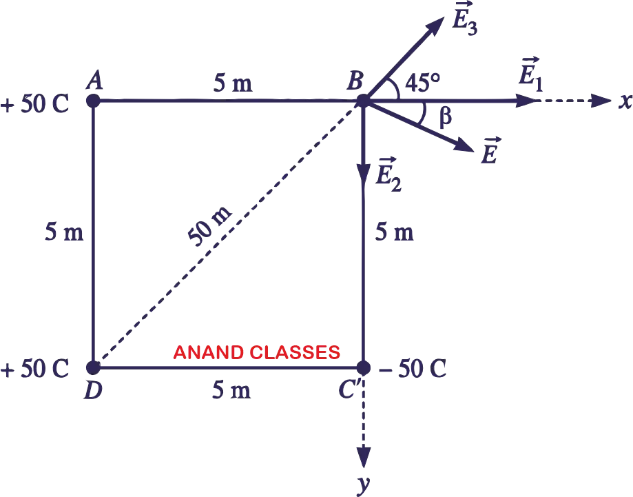
Solution. Electric field at B due to +50 C charge at A is

$E_1 = k cdot dfrac{q}{r^2} = k cdot dfrac{50}{5^2} = 2k, text{ along } AB$

Electric field at B due to -50 C charge at C is

$E_2 = k cdot dfrac{50}{5^2} = 2k, text{ along } BC$

Electric field at B due to +50 C charge at D is

$E_3 = k cdot dfrac{50}{left(sqrt{5^2 + 5^2}right)^2} = k, text{ along } DB$

Component of E₁ along x-axis = 2k (as it acts along x-axis)

Component of E₂ along x-axis = 0 (as it acts along y-axis)

Component of E₃ along x-axis $= E_3 cos 45^circ = k cdot dfrac{1}{sqrt{2}} = dfrac{k}{sqrt{2}}$

Therefore total electric field at B along x-axis,

$E_x = 2k + 0 + dfrac{k}{sqrt{2}} = k left( 2 + dfrac{1}{sqrt{2}} right)$

Now,

Component of E₁ along y-axis = 0

Component of E₂ along y-axis = 2k

Component of E₃ along y-axis $E_y = E_3 sin 45^circ = k cdot dfrac{1}{sqrt{2}} = dfrac{k}{sqrt{2}}$

But the components of E₂ and E₃ act in opposite directions, therefore, total electric field at B along y-axis

$$= 2k – dfrac{k}{sqrt{2}} = k left( 2 – dfrac{1}{sqrt{2}} right)$$

Therefore resultant electric field at B will be

$E = sqrt{E_x^2 + E_y^2}$

$E = sqrt{left[ k left( 2 + dfrac{1}{sqrt{2}} right) right]^2 + left[ k left( 2 – dfrac{1}{sqrt{2}} right) right]^2} = sqrt{9k^2}$

$E = 3k = 3 times 9 times 10^9text{ NC}^{-1} = 2.7 times 10^{10}text{ NC}^{-1}$

If the resultant field E makes angle β with x-axis, then

$tan beta = dfrac{E_y}{E_x} = dfrac{(2 – 1/sqrt{2})k}{(2 + 1/sqrt{2})k} = 0.4776 quad text{or} quad beta = 25.5^circ$

---

Four charges +q, +q, –q, –q are placed respectively at the four corners A, B, C and D of a square of side ‘a’. Calculate the electric field at the centre of the square.

Solution. Let E_A, E_B, E_C and E_D be the electric fields at the centre O of the square due to the charges at A, B, C and D respectively. Their directions are as shown in Figure.a.

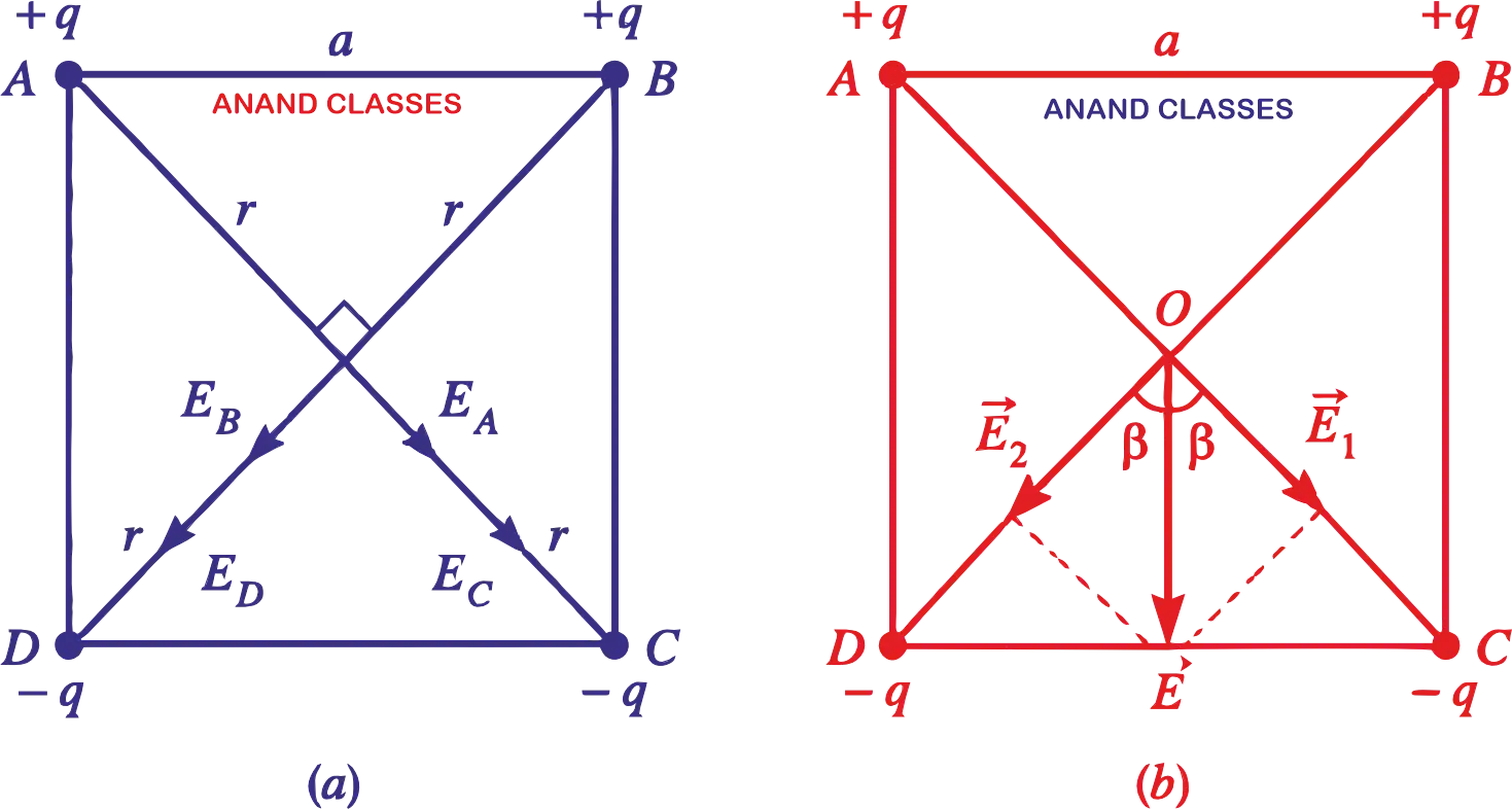
Since all the charges are of equal magnitude and at the same distance r from the centre O, so

$E_A = E_B = E_C = E_D = k cdot dfrac{q}{r^2}$

$= dfrac{kq}{left( dfrac{a}{sqrt{2}} right)^2} = dfrac{2kq}{a^2} quad left[because r^2 + r^2 = a^2right]$

Because E_A and E_C act in the same direction, so their resultant is

$E_1 = E_A + E_C = dfrac{2kq}{a^2} + dfrac{2kq}{a^2} = dfrac{4kq}{a^2}$

Similarly, resultant of E_B and E_D is

$E_2 = E_B + E_D = dfrac{4kq}{a^2}$

Now, the resultant of E₁ and E₂ will be

$E = sqrt{E_1^2 + E_2^2}$

$E = sqrt{left(dfrac{4kq}{a^2}right)^2 + left(dfrac{4kq}{a^2}right)^2} = 4sqrt{2}k dfrac{q}{a^2}$

directed parallel to AD or BC, as shown in Figure.(b).

$cos beta = dfrac{E_1}{E} = dfrac{1}{sqrt{2}} implies beta = 45^circ$

i.e., the resultant field is inclined at an angle of 45° with AC.

---

Two point charges +6q and -8q are placed at the vertices ‘B’ and ‘C’ of an equilateral triangle ABC of side ‘a’ as shown in Figure(a). Obtain the expression for
(i) the magnitude and
(ii) the direction of the resultant electric field at the vertex A due to these two charges.

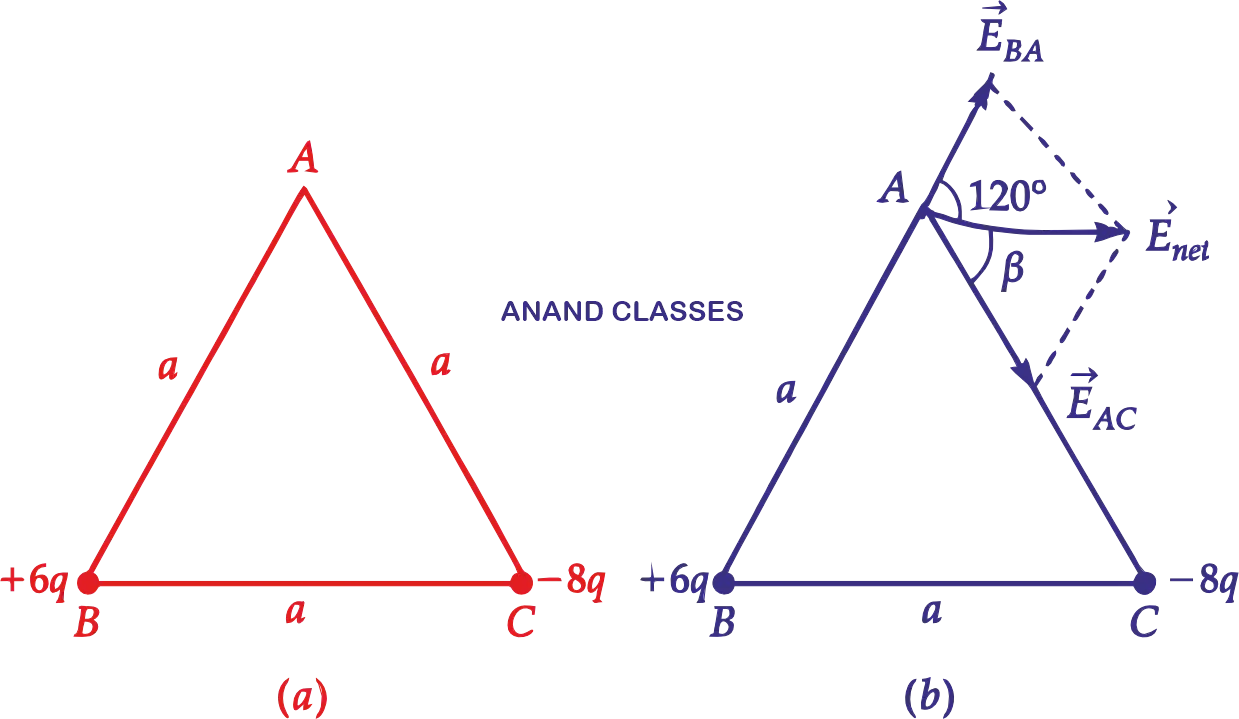
Solution. (i) As shown in Figure(b), the fields at point A due to the charges at B and C are $vec{E}_{BA}$ and $vec{E}_{AC}$ respectively.

Their magnitudes are :

$E_{BA} = dfrac{1}{4pivarepsilon_0} dfrac{6q}{a^2} = 6E,$

$text{where } E = dfrac{1}{4pivarepsilon_0} dfrac{q}{a^2}$

$E_{AC} = dfrac{1}{4pivarepsilon_0} dfrac{8q}{a^2} = 8E$

The magnitude of the resultant field is :

$E_{text{net}} = sqrt{E_{BA}^2 + E_{AC}^2 + 2 E_{BA} E_{AC} cos 120^circ}$

$= sqrt{(6E)^2 + (8E)^2 + 2 times 6E times 8E times left(-dfrac{1}{2}right)}$

$= Esqrt{52} = dfrac{1}{4pivarepsilon_0} dfrac{qsqrt{52}}{a^2}$

(ii) If the resultant field makes an angle β with AC, then

$tan beta = dfrac{E_{BA} sin 120^circ}{E_{AC} + E_{BA} cos 120^circ}$

$tan beta = dfrac{6E times (sqrt{3}/2)}{8E + 6E times (-1/2)} = dfrac{3sqrt{3}}{5}$

$therefore beta = tan^{-1} left( dfrac{3sqrt{3}}{5} right)$

---