Applications of Gauss’s Law: Electric Field due to Infinitely long Charged Wire & Cylinder, Numericals

Application of Gauss’s Law – Electric field due to an infinitely long straight uniformly charged wire is an important topic in CBSE Class 12 Physics Electrostatics and is also useful for JEE and NEET preparation. In this chapter, we derive the electric field of an infinite line charge using Gauss’s law, understand the role of a cylindrical Gaussian surface, and study how electric field varies with perpendicular distance from the charged wire. The topic also forms the basis for solving numerical problems involving linear charge density, electric flux, charged cylinders, electric dipoles, and applications of Gauss’s theorem.

Electrostatics Complete Revision Notes PDF Download : Electric Field due to Infinitely long Charged Wire & Charged Cylinder Using Gauss’s Law

Download the Electrostatics Complete Revision Notes PDF covering Electric Field due to Infinitely long Charged Wire & Charged Cylinder, including important concepts, formulas, key results, and exam-focused points for CBSE Class 12, JEE, and NEET preparation.

To download the PDF notes of Electric Field due to Infinitely long Charged Wire & Charged Cylinder, click the Download PDF button below :

---

Derivation of Electric Field due to an Infinitely long Straight Uniformly Charged Wire Using Gauss’s Law

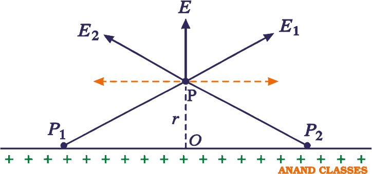
Consider an infinitely long thin wire carrying a uniform linear charge density λ. To evaluate the electric field intensity at an arbitrary observation point P, select a pair of symmetric line elements P₁ and P₂ placed at equal distances from a designated origin O on the wire.

Electric fields $\vec{E}_1$ and $\vec{E}_2$ at point P due to the two line elements are shown in Figure. Their components normal to the radius vector OP = r cancel out, being equal and opposite. However, the components along OP add. Therefore, resultant electric field is radial. This is true for any such pair of line elements. Therefore, total field at any point P is radial. As the wire is infinite, electric field does depend upon distance of point from the wire, but not on the position of P. Thus, electric field at every point in the plane cutting the wire normally is radial; and its magnitude depends only on the radial distance r.

To determine the electric field at a distance r from a line charge, we choose a cylindrical Gaussian surface of radius r, length l, and with its axis along the line charge.

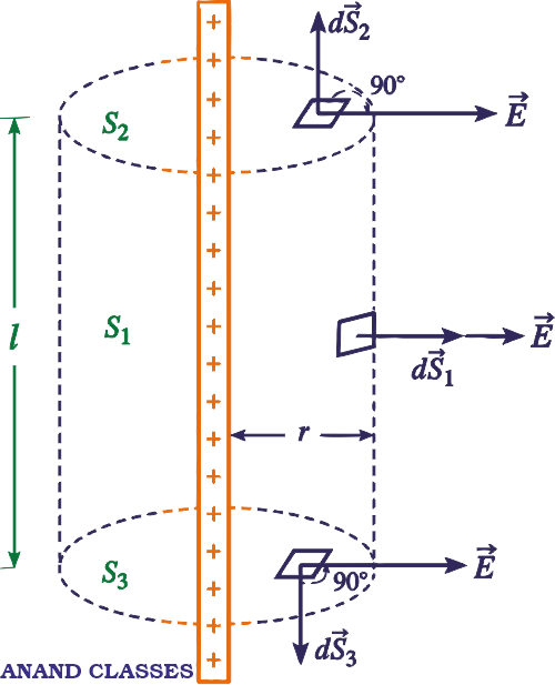
As shown in Figure, it has a curved surface S₁ and flat circular ends S₂ and S₃. Obviously, d$\vec{S_1}\parallel \vec{E}$, d$\vec{S_2}\perp \vec{E}$, and d$\vec{S_3}\perp \vec{E}$. So only the curved surface contributes towards the total flux.

$$\phi = \oint_{S}\vec{E}\cdot\vec{ds}$$

$$\phi = \int_{S_1} \vec{E} \cdot d\vec{S_1} + \int_{S_2} \vec{E} \cdot d\vec{S_2} + \int_{S_3} \vec{E} \cdot d\vec{S_3}$$

$$\phi = \int_{S_1} E \, dS_1 \cos 0^\circ + \int_{S_2} E \, dS_2 \cos 90^\circ + \int_{S_3} E \, dS_3 \cos 90^\circ$$

$$\phi = E \int_{S_1} dS_1 + 0 + 0$$

ϕ = E × area of the curved surface of cylinder

ϕ = E × 2πrl

∴ Total electric flux over the whole cylinder, ϕ_E = E(2πrl)

Charge enclosed in the cylinder = linear charge density × length of cylinder

q = λl

According to Gauss’s theorem,

$$\phi_{E}=\frac{q}{\epsilon_{0}}$$

$$E(2\pi rl)=\frac{\lambda l}{\epsilon_{0}}$$

$$E=\frac{\lambda}{2\pi\epsilon_{0}r}$$

E ∝ 1/r

If λ > 0, the direction of electric field at every point is radially outwards. If λ < 0, the direction of electric field at every point is radially inwards.

Strengthen your fundamentals with Electric Flux & Gauss’s Law, Numericals, Questions & Answers

Derivation of Electric Field between a Charged Cylinder and a Coaxial Conducting Cylinder Using Gauss’s Law

A long charged cylinder of linear charge density is surrounded by a co-axial conducting cylinder. The electric field in the space between the two cylinders is compute as follows :

Figure. shows a long charged cylinder A surrounded by a co-axial cylindrical shell B. Let l be the common length of the cylinder and the cylindrical shell. When charge +q is given to the inner cylinder A, charge equal to –q is induced on the inner surface of the cylindrical shell B and charge +q on its outer surface.

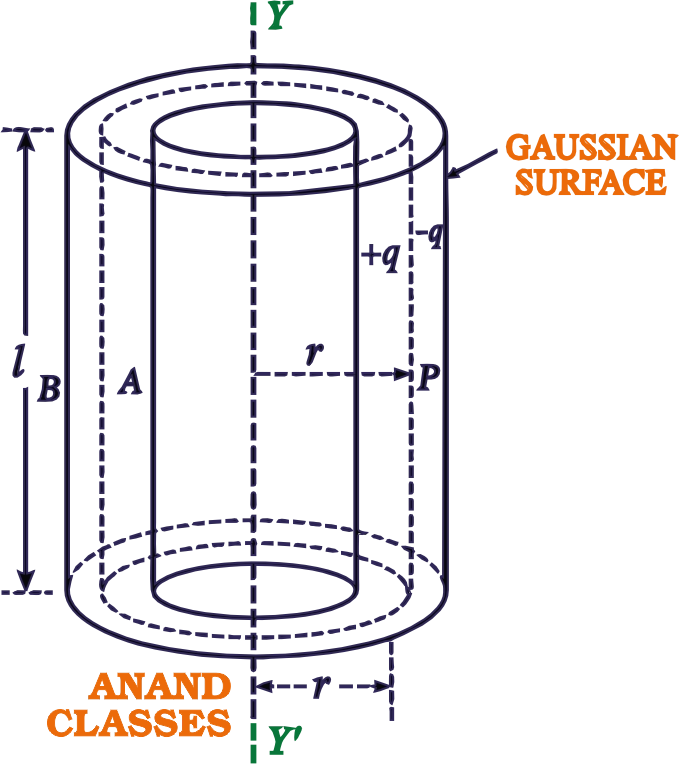
The electric field in the space between the two cylinders is not uniform. Let E be the electric field at any point P at a distance r from the axis of the cylinder A.

To find the value of electric field E, draw a cylindrical shell of radius r through point P as the gaussian surface as shown in the figure. It encloses charge q on the inner cylindrical shell A.

According to Gauss’ theorem, the total electric flux through the gaussian surface,

$$\phi_{E}=\frac{q}{\epsilon_{0}}$$

As the magnitude of electric field at every point on the gaussian surface is same, we have total electric flux of gaussian surface of cylinder

ϕ = E × surface area of gaussian surface of cylinder

ϕ = E × 2πrl

$$E \times 2\pi rl = \dfrac{q}{\varepsilon_0}$$

$$E = \dfrac{q}{2\pi \varepsilon_0 rl}$$

If λ is linear charge density of the cylinder A, then

q = λ l

$$E = \dfrac{\lambda}{2\pi \varepsilon_0 r}$$

Frequently linked concepts include Electric Dipole Moment, Electric Field on Axial and Equatorial Line of Electric Dipole and on axis of Uniformly Charged Ring with Numericals

---

Noteworthy Points for CBSE Class 12 Physics, JEE and NEET

1. In the above derivation, electric field is due to charge on the entire wire of infinite length. However, the charge enclosed by the cylindrical Gaussian surface is only λ × l.
2. The assumption that the wire is infinitely long is crucial. Direction of electric filed (E) is taken normal to the curved part of the cylindrical Gaussian surface only on account of this assumption.
3. If the wire is not infinitely long, we have to take into consideration the end effects.

Explore more concepts related to Electric Field Lines Properties, Electric Field due to Infinitely long thin wire, Charged Circular and Semicircular Ring

---

Solved Numerical Problems on Applications of Gauss’s Law – Electric Field due to Infinitely long Charged Wire & Cylinder

Solved numerical problems based on applications of Gauss’s Law – Electric Field due to Infinitely long Charged Wire & Cylinder help students apply Gauss’s law, electric field formulas, electric flux, and linear charge density to CBSE Class 12 Physics, JEE, and NEET-level questions.

An infinite line charge produces a field of 9 × 10⁴ N C⁻¹ at a distance of 0.02 m. Calculate the linear charge density.

Sol. Here, E = 9 × 10⁴ N C⁻¹, r = 0.02 m, λ = ?

As

$$E = \frac{\lambda}{2\pi\epsilon_{0}r}$$

$$E =\frac{2\lambda}{4\pi\epsilon_{0}r}$$

$$\lambda=\frac{E\times 4\pi\epsilon_{0}r}{2}$$

$$\lambda=9\times 10^{4}\times\frac{1}{9\times 10^{9}}\times\frac{0.02}{2}$$

λ = 10⁻⁷ C m⁻¹

A plastic rod of length 2.2 m and radius 3.6 mm carries a negative charge of -3.8 x 10⁻⁸ C spread uniformly over its surface. What is the electric field near the mid-point of the rod, at a point on its surface?

Solution : Given, Length of the rod (l) = 2.2 m, Radius of the rod (r) = 3.6 mm = 3.6 x 10⁻³ m, Total charge (q) = -3.8 x 10⁻⁸ C

The linear charge density of the rod is :

λ = q / l

λ = (-3.8 x 10⁻⁸) / (2.2 m) = -1.73 x 10⁻⁸ C/m

Near the mid-point of the rod, at a point on its surface, the rod can be treated approximately as an infinite line charge. The electric field E due to a line charge is given by :

E = [1 / (4πε₀)] × (2 × λ / r)

Substituting the known values into the formula:

E = (9 x 10⁹) × 2 × (-1.73 x 10⁻⁸) / (3.6 x 10⁻³)

E = -8.6 x 10⁴ N/C

The electric field near the mid-point on the surface of the rod has a magnitude of 8.6 x 10⁴ N/C and is directed radially inward toward the rod because the charge is negative.

Calculate the total flux of the electrostatic field through the spheres S₁ and S₂. The wire AB shown here has a linear charge density λ given by λ = kx, where x is the distance measured along the wire from end A.

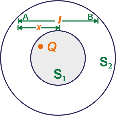
Solution. Charge on an element of length dx of wire AB

dq = λ dx = kx dx

Total charge on wire AB,

$$q = \int dq = \int_0^l kx \, dx$$

$$q = k \left( \frac{x^2}{2} \right)_0^l$$

$$q = \frac{1}{2} kl^2$$

Total flux through $S_1 = \phi_1 = \dfrac{Q}{\in_0}$

Total flux through $S_2 = \phi_2 = \dfrac{Q + q}{\in_0}$

$$\phi_2 = \dfrac{Q + \dfrac{1}{2} kl^2}{\in_0}$$

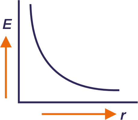
Draw a graph to show the variation of electric intensity E with perpendicular distance r from an infinite line of charge density λ C/m. Find work done in bringing a charge q from perpendicular distance r₁ to r₂ (r₂ > r₁).

Solution : As is known, electric intensity E at a perpendicular distance r from an infinite line of charge density λ C/m is

E = λ / (2πε₀r)

The variation of E with r is as shown in Figure.

Work done in bringing charge q from distance r₁ to r₂ is

$$dW = \Sigma F \, dr$$

$$dW = qE \, dr$$

$$dW = q \frac{\lambda}{2\pi \in_0 r} \, dr$$

$$W = \int_{r_1}^{r_2} \frac{\lambda q}{2\pi \in_0 r} \, dr$$

$$W = \frac{\lambda q}{2\pi \in_0} [\log r]_{r_1}^{r_2}$$

$$W = \frac{\lambda q}{2\pi \in_0} \log \left( \frac{r_2}{r_1} \right)$$

Students should also study Electric Charge Quantization, Additivity, Charging by Induction, Solved Numericals

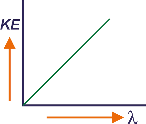
(a) An infinitely long positively charged wire has a linear charge density λ C/m. An electron is revolving around the wire as its centre with a constant velocity in a circular plane perpendicular to the wire. Deduce the expression for its kinetic energy. (b) Plot a graph of the kinetic energy as a function of charge density λ.

Solution. The electrostatic force exerted by the line charge on the electron provides the centripetal force for the revolution of electron. Therefore,

Force exerted by electric field = Centripetal force

eE = mv²/r

Here v is the orbital velocity of the electron

But

E = λ / (2πε₀r)

Therefore,

(e λ) / (2πε₀r) = mv²/r

v² = (e λ) / (2πε₀m)

Kinetic energy of the electron will be

KE = 1/2 mv²

KE = (e λ) / (4πε₀)

KE ∝ λ

(b) As KE ∝ λ, the graph of kinetic energy KE vs. charge density λ will be a straight line as shown in Figure.

Two long straight parallel wires carry charges λ₁ and λ₂ per unit length. The separation between their axes is d. Find the magnitude of the force exerted on unit length of one due to the charge on the other.

Solution. Electric field at the location of wire 2 due to charge on 1 is

E = λ₁ / (2πε₀d)

Force per unit length of wire 2 due to the above field

F = E × charge on unit length of wire₂

F = E λ₂

F = λ₁ λ₂/ (2πε₀d)

An electric dipole consists of charges ±2 ×10⁻⁸ C, separated by a distance of 2 mm. It is placed near a long line charge of density 4.0 × 10⁻⁴ C/m, as shown in Figure, such that the negative charge is at a distance of 2 cm from the line charge. Calculate the force acting on the dipole.

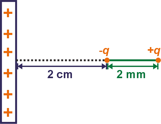
Solution. Electric field due to a line charge at distance r from it,

E = [1 / (4πε₀)] × (2 × λ / r)

Force exerted by this field on charge q,

F = qE

F = [1 / (4πε₀)] × (2 × λq / r)

Force exerted on negative charge (r = 0.02 m),

F₁ = (9 × 10⁹) × (2 × 2 × 10⁻⁸ × 4 × 10⁻⁴)/0.02 N

F₁ = 7.2 N, acting towards the line charge

Force exerted on positive charge r = 2.2 × 10⁻² m,

F₂ = (9 × 10⁹) × (2 × 2 × 10⁻⁸ × 4 × 10⁻⁴)/(2.2 × 10⁻²) N

F₂ = 6.5 N, acting away from the line charge

Net force on the dipole,

F = F₁- F₂

F = 7.2 – 6.5

F = 0.7 N, acting towards the line charge.

A thin straight rod of length L has uniform linear charge density λ. Moving at a constant speed v, the rod enters a cube of sides having length L through its left face and leaves through the right face as shown in Figure.
(i) Find the maximum electric flux through the cube.
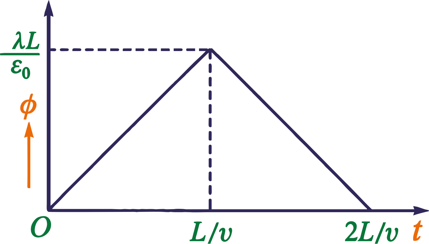
(ii) Graphically, represent the variation of electric flux through the cube with time between the instants, the rod just begins to enter and when it leaves the cube.

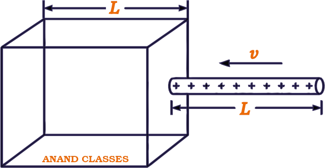
(i) The electric flux through the cube will be maximum, when it encloses the maximum charge i.e. when the rod is completely inside the cube.

The charge on whole length of the rod,

Q = λL

Hence, the maximum electric flux through the cube,

ϕ = Q/ε₀

ϕ = (λL)/ε₀

(ii) At any time t, length of the rod inside the cube = v t
Therefore, at any time t, the charge inside the cube,

q_t = λ(vt)

Hence, electric flux linked with the cube at any time t,

ϕ_t = q_t/ε₀

ϕ_t = (λvt)/ε₀

ϕ_t ∝ t

Therefore, electric flux linked with the cube will vary linearly with time, increasing from zero to the maximum value during the time interval between 0 to L/v and then decreasing from the maximum value to zero during the time interval between L/v to 2 L/v shown in Figure.

A thin straight rod of length 2L has uniform linear charge density λ. Moving at a constant speed v, the rod enters a cube of sides having length L through its left face and leaves through the right face, then
(i) find the maximum electric flux through the cube and
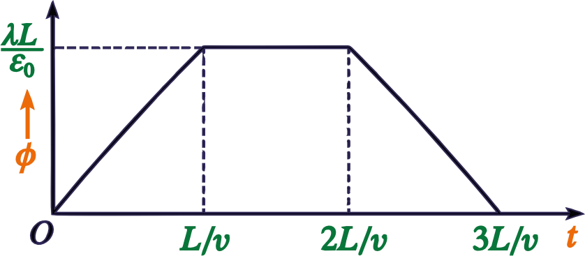
(ii) graphically, represent the variation of electric flux through the cube with time between the instants, the rod just begins to enter and when it leaves the cube.

(i) Since side of the cube is L, the maximum length of the rod, which can be inside the cube will also be L. Hence, the maximum electric flux through the cube will remain the same

ϕ = (λL)/ε₀

As already proved in above question, the electric flux linked with the cube will vary linearly with time, increasing from zero to the maximum value during the time interval between 0 to L/v; remaining unchanged during the time interval L/v to 2L/v and then decreasing from the maximum value to zero during the time interval 2L/v to 3L/v as shown in Figure.

Also study Electric Field due to Point Charge, Group of Charges, Continuous Charge Distribution Numerical Problems

---

Very Short Frequently Asked Questions (FAQs) and Answers

Test your understanding of electric field, Gauss’s law, electric flux, linear charge density, and the field due to an infinitely long charged wire through concise conceptual questions for Class 12 Physics, JEE, NEET exams.

Does the strength of electric field due to an infinitely long line charge depend upon the distance of the observation point from the line charge ?

Yes, the electric field due to an infinitely long line charge depends upon the distance of the observation point from the line charge.

How does electric field at a point change with distance r from an infinitely long charged wire ?

The electric field varies inversely with the perpendicular distance r, E ∝ 1/r. Therefore, the field decreases as the distance from the wire increases.

What is the direction of the electric field due to an infinite line charge?

For positive linear charge density, the electric field is radially outward. For negative linear charge density, it is radially inward.

Why is the electric field radial for an infinitely long charged wire?

For symmetric pairs of charge elements, the components perpendicular to the radius vector cancel, while the components along the radius vector add. Hence, the resultant electric field is radial.

What Gaussian surface is used for an infinitely long line charge?

A cylindrical Gaussian surface with radius r, length l, and its axis along the charged wire is used.

Why is the assumption of an infinitely long wire important?

The infinite-wire assumption allows the electric field to be treated as radial and normal to the curved surface of the cylindrical Gaussian surface. For a finite wire, end effects must be considered.

Learn more about Applications of Gauss’s Law: Electric Field due to Infinitely long Charged Wire & Cylinder, Numericals

---

Electrostatics Complete Revision Notes PPTX Slideshow Presentation Download: Electric Field due to Infinitely long Charged Wire & Charged Cylinder

Download the Electrostatics Complete Revision Notes PPTX Slideshow on Electric Field due to Infinitely long Charged Wire & Charged Cylinder, featuring important concepts, formulas, key results, and exam-focused content for CBSE Class 12, JEE, and NEET preparation.

To download the PPTX Slideshow Presentation notes of Electric Field due to Infinitely long Charged Wire & Charged Cylinder, click the Download Slideshow PPTX Presentation button below :

Enhance your preparation with Forces Between Multiple Charges: Principle of Superposition Solved Numerical Problems

---

Electrostatics: Electric Field due to Infinitely long Charged Wire & Charged Cylinder Using Gauss’s Law Presentation Video

Watch the video to understand Electric Field due to Infinitely long Charged Wire & Charged Cylinder Using Gauss’s Law through important concepts, solved numericals, and short questions with answers, specially useful for CBSE Class 12, JEE, and NEET preparation.

For complete preparation, also study Coulomb’s Law of Electrostatics: Formula, Vector Form, Examples & Numericals